How do language models solve Bayesian network inference?
Table of Contents
Can language models think "probabilistically"?
This question has been on my mind for a while. It motivated me to revisit probabilistic graphical models, write my blog series on Decision Theory, and explore how large language models (LLMs) solved a few hand-crafted decision problems.
Early experiments were promising: models like O3 and Gemini-2.5-Pro reached correct solutions on small decision problems. But I observed they were solving them using decision trees, which have theoretical limitations. I wondered: were LLMs using decision trees because it was “easier”, or because they didn’t know how to apply influence diagrams?
To answer that, I started running more extensive experiments. But midway through, I realized I was getting ahead of myself. If I wanted to evaluate LLMs on influence diagrams, I should probably start with Bayesian networks, since influence diagrams are essentially Bayesian networks augmented with decisions and utilities. If LLMs struggle with probabilistic inference on Bayesian networks, expecting them to solve full decision problems could be premature.
So that’s what this post explores: how do current frontier LLMs handle probabilistic inference on a Bayesian network? I’ll walk through the Variable Elimination algorithm since it is one of the easiest to understand and implement, solve an example by hand with it, and then compare how seven reasoning LLMs approach the same query, analyzing not just whether they get the right answer, but how they reason through the problem.
Bayesian networks
A Bayesian network (BN) is a directed acyclic graph (DAG) in which nodes represent random variables. Arcs encode conditional dependencies between variables in a way that allows us to factorize the joint probability distribution into a product of conditional probability distributions (CPDs),
\[\begin{equation} P(\mathbf{\textcolor{purple}{V}}) = P(\textcolor{purple}{V_1}, \ldots, \textcolor{purple}{V_n}) = \prod_{i=1}^{n} P(\textcolor{purple}{V_i} | \mathbf{Pa}_{\textcolor{purple}{V_i}}) \end{equation}\]where \(\mathbf{Pa}_{\textcolor{purple}{V_i}}\) denotes the parents of variable \(\textcolor{purple}{V_i}\) in the DAG. This property is often called the chain rule for Bayesian networks.
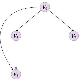
As an example, consider a Bayesian network with 4 binary variables (\(\textcolor{purple}{V_0}, \textcolor{purple}{V_1}, \textcolor{purple}{V_2}, \textcolor{purple}{V_3}\)). The structure is a simple diamond-like shape where \(\textcolor{purple}{V_0}\) is the root, \(\textcolor{purple}{V_1}\) and \(\textcolor{purple}{V_2}\) depend on \(\textcolor{purple}{V_0}\), and \(\textcolor{purple}{V_3}\) depends on both \(\textcolor{purple}{V_0}\) and \(\textcolor{purple}{V_1}\).
|
|
| Figure 1. Bayesian network example with 4 variables | |
| $$P(\textcolor{purple}{V_0})$$ | |
|---|---|
| $$\textcolor{purple}{s_0}$$ | 0.5072 |
| $$\textcolor{purple}{s_1}$$ | 0.4928 |
| $$P(\textcolor{purple}{V_1} \mid \textcolor{purple}{V_0})$$ | $$\textcolor{purple}{V_0}$$ | |
|---|---|---|
| $$\textcolor{purple}{s_0}$$ | $$\textcolor{purple}{s_1}$$ | |
| $$\textcolor{purple}{s_0}$$ | 0.3110 | 0.0704 |
| $$\textcolor{purple}{s_1}$$ | 0.6890 | 0.9296 |
| $$P(\textcolor{purple}{V_2} \mid \textcolor{purple}{V_0})$$ | $$\textcolor{purple}{V_0}$$ | |
|---|---|---|
| $$\textcolor{purple}{s_0}$$ | $$\textcolor{purple}{s_1}$$ | |
| $$\textcolor{purple}{s_0}$$ | 0.8950 | 0.0562 |
| $$\textcolor{purple}{s_1}$$ | 0.1050 | 0.9438 |
| $$P(\textcolor{purple}{V_3} \mid \textcolor{purple}{V_0},\, \textcolor{purple}{V_1})$$ | $$\textcolor{purple}{V_0 = s_0}$$ | $$\textcolor{purple}{V_0 = s_1}$$ | ||
|---|---|---|---|---|
| $$\textcolor{purple}{V_1 = s_0}$$ | $$\textcolor{purple}{V_1 = s_1}$$ | $$\textcolor{purple}{V_1 = s_0}$$ | $$\textcolor{purple}{V_1 = s_1}$$ | |
| $$\textcolor{purple}{s_0}$$ | 0.0607 | 0.8173 | 0.8890 | 0.2251 |
| $$\textcolor{purple}{s_1}$$ | 0.9393 | 0.1827 | 0.1110 | 0.7749 |
Probabilistic inference on Bayesian networks
Once we have a BN, we can use it to reason by performing probabilistic inference. This task involves computing the probability of query variables \(\mathbf{\textcolor{purple}{Q}}\) given some observed evidence \(\mathbf{\textcolor{purple}{E}} = \mathbf{\textcolor{purple}{e}}\).
Theoretically, this is straightforward. The Bayesian network defines the full joint distribution, so we could sum over all unobserved “nuisance” variables \(\mathbf{\textcolor{purple}{Z}}\):
\[\begin{equation} P(\mathbf{\textcolor{purple}{Q}} = \mathbf{\textcolor{purple}{q}} \mid \mathbf{\textcolor{purple}{E}} = \mathbf{\textcolor{purple}{e}}) = \frac{\sum_{\mathbf{\textcolor{purple}{z}}} P(\mathbf{\textcolor{purple}{Q}} = \mathbf{\textcolor{purple}{q}}, \mathbf{\textcolor{purple}{E}} = \mathbf{\textcolor{purple}{e}}, \mathbf{\textcolor{purple}{Z}} = \mathbf{\textcolor{purple}{z}})}{\sum_{\mathbf{\textcolor{purple}{q}}, \mathbf{\textcolor{purple}{z}}} P(\mathbf{\textcolor{purple}{Q}} = \mathbf{\textcolor{purple}{q}}, \mathbf{\textcolor{purple}{E}} = \mathbf{\textcolor{purple}{e}}, \mathbf{\textcolor{purple}{Z}} = \mathbf{\textcolor{purple}{z}})} \end{equation}\]However, this naive approach is computationally infeasible. For a network with \(n\) binary variables, storing the full joint distribution would require a table with \(2^n\) entries.
Instead of storing that massive table, we can use the BN factorization (Equation 1) to compute only the specific joint probabilities we need on-the-fly. By substituting the factorization into Equation (2), we get:
\[\begin{equation} P(\mathbf{\textcolor{purple}{Q}} = \mathbf{\textcolor{purple}{q}} \mid \mathbf{\textcolor{purple}{E}} = \mathbf{\textcolor{purple}{e}}) = \frac{\sum_{\mathbf{\textcolor{purple}{z}}} \prod_{i=1}^{n} P(\textcolor{purple}{V_i} \mid \mathbf{Pa}_{\textcolor{purple}{V_i}})}{\sum_{\mathbf{\textcolor{purple}{q}}, \mathbf{\textcolor{purple}{z}}} \prod_{i=1}^{n} P(\textcolor{purple}{V_i} \mid \mathbf{Pa}_{\textcolor{purple}{V_i}})} \end{equation}\]While this saves us from storing the full table, we still face the problem of summing over it. We still need to enumerate all combinations of hidden variables \(\mathbf{\textcolor{purple}{z}}\). For 30 binary variables, that’s over a billion terms to sum. This approach, often called inference by enumeration or simply applying the chain rule naively, is conceptually simple but does not scale.
Efficient inference algorithms avoid this exponential blowup by exploiting the factorized representation more cleverly. Rather than enumerating all combinations, they manipulate the individual CPDs (which are much smaller) and perform marginalization locally, pushing sums inside products where conditional independence allows. Well-known examples include Variable Elimination, Junction Tree algorithm, and Belief Propagation (Koller & Friedman, 2009). We’ll focus on Variable Elimination since it’s the easiest to explain and commonly used when teaching BN inference.
Variable Elimination algorithm
As the name suggests, the Variable Elimination (VE) algorithm works by eliminating the variables of the network until it yields the answer to a specific query. This algorithm is typically defined in terms of factors.
A factor \(\phi(\mathbf{\textcolor{purple}{X}})\) is a function that maps a set of variables \(\mathbf{\textcolor{purple}{X}}\) to a real positive value. CPDs are an example of factors. In fact, the initial set of factors corresponds exactly to the CPDs of the network.
During inference, new factors are created by multiplying and marginalizing existing ones. These intermediate factors are generally unnormalized, meaning their values do not sum to one. This is not a problem, since normalization is only required for the final result. Working with unnormalized factors simplifies computation and allows inference algorithms to focus on local operations.
Operations on factors
VE relies on three operations:
- Factor Product: Combine two factors \(\phi_1(\textcolor{purple}{V_1})\) and \(\phi_2(\textcolor{purple}{V_2})\) into a new factor \(\phi_{new}\) over \(\textcolor{purple}{V_1} \cup \textcolor{purple}{V_2}\) by multiplying their values for every consistent assignment:
-
Marginalization: Eliminate a variable \(\textcolor{purple}{Z}\) from factor \(\phi(\textcolor{purple}{V}, \textcolor{purple}{Z})\) by summing over all its values to produce a new factor \(\phi_{new}\):
\[\phi_{new}(\textcolor{purple}{V}) = \sum_{\textcolor{purple}{z}} \phi(\textcolor{purple}{V}, \textcolor{purple}{Z} =\textcolor{purple}{z})\] -
Evidence restriction: If variable \(\textcolor{purple}{E}\) is observed to be \(\textcolor{purple}{e}\), restrict any factor containing \(\textcolor{purple}{E}\) to that value, essentially selecting the slice of the table consistent with the observation.
The algorithm
Given a Bayesian network, query variables \(\mathbf{\textcolor{purple}{Q}}\), and evidence \(\mathbf{\textcolor{purple}{E}} = \mathbf{\textcolor{purple}{e}}\):
-
Initialize: Treat each CPD as a factor. Restrict all factors to be consistent with the evidence \(\mathbf{\textcolor{purple}{E}} = \mathbf{\textcolor{purple}{e}}\).
-
Choose elimination order: Pick an ordering for the hidden variables \(\mathbf{\textcolor{purple}{Z}}\) (neither query nor evidence). The choice of ordering affects efficiency because bad orders create large intermediate factors.
- Eliminate variables: For each variable \(\textcolor{purple}{Z_i}\) in order:
- Collect all factors containing \(\textcolor{purple}{Z_i}\)
- Multiply them into a single factor \(\phi_{new}'\)
- Sum out \(\textcolor{purple}{Z_i}\) to get a new factor \(\phi_{new}''\)
- Replace the collected factors with \(\phi_{new}''\)
- Normalize: Multiply remaining factors (now only over \(\mathbf{\textcolor{purple}{Q}}\)) and normalize to obtain \(P(\mathbf{\textcolor{purple}{Q}} = \mathbf{\textcolor{purple}{q}} \mid \mathbf{\textcolor{purple}{E}} = \mathbf{\textcolor{purple}{e}})\).
Example
As an example we are going to use the BN we defined in Figure 1 and compute the probability of \(\textcolor{purple}{V_3}\) being \(\textcolor{purple}{s_1}\) given that \(\textcolor{purple}{V_1}\) is observed to be \(\textcolor{purple}{s_0}\):
\[P(\textcolor{purple}{V_3} = \textcolor{purple}{s_1} \mid \textcolor{purple}{V_1} = \textcolor{purple}{s_0})\]The evidence is \(\mathbf{\textcolor{purple}{E}} = \{\textcolor{purple}{V_1} = \textcolor{purple}{s_0}\}\). The query variable is \(\mathbf{\textcolor{purple}{Q}} = \{\textcolor{purple}{V_3}\}\). The hidden variables to eliminate are \(\mathbf{\textcolor{purple}{Z}} = \{\textcolor{purple}{V_0}, \textcolor{purple}{V_2}\}\).
We start with the initial factors (the CPDs):
\[\begin{aligned} \phi_0(\textcolor{purple}{V_0}) &= P(\textcolor{purple}{V_0}) \\ \phi_1(\textcolor{purple}{V_1}, \textcolor{purple}{V_0}) &= P(\textcolor{purple}{V_1} \mid \textcolor{purple}{V_0}) \\ \phi_2(\textcolor{purple}{V_2}, \textcolor{purple}{V_0}) &= P(\textcolor{purple}{V_2} \mid \textcolor{purple}{V_0}) \\ \phi_3(\textcolor{purple}{V_3}, \textcolor{purple}{V_0}, \textcolor{purple}{V_1}) &= P(\textcolor{purple}{V_3} \mid \textcolor{purple}{V_0}, \textcolor{purple}{V_1}) \end{aligned}\]For the elimination order, we have randomly selected to start with \(\textcolor{purple}{V_2}\) and then \(\textcolor{purple}{V_0}\).
Step 1: Restrict factors based on evidence
Since we observe \(\textcolor{purple}{V_1} = \textcolor{purple}{s_0}\), we restrict any factor containing \(\textcolor{purple}{V_1}\) to this value.
For \(\phi_1(\textcolor{purple}{V_1}, \textcolor{purple}{V_0})\), we fix \(\textcolor{purple}{V_1} = \textcolor{purple}{s_0}\). Since \(\textcolor{purple}{V_1}\) is now a constant, the resulting factor depends only on \(\textcolor{purple}{V_0}\). We call this new factor \(\phi_1'(\textcolor{purple}{V_0})\):
| $$\phi_1'(\textcolor{purple}{V_0})$$ | |
|---|---|
| $$\textcolor{purple}{s_0}$$ | 0.3110 |
| $$\textcolor{purple}{s_1}$$ | 0.0704 |
For \(\phi_3(\textcolor{purple}{V_3}, \textcolor{purple}{V_0}, \textcolor{purple}{V_1})\), we similarly select the entries consistent with \(\textcolor{purple}{V_1} = \textcolor{purple}{s_0}\). The new factor depends only on \(\textcolor{purple}{V_3}\) and \(\textcolor{purple}{V_0}\):
| $$\phi_3'(\textcolor{purple}{V_3}, \textcolor{purple}{V_0})$$ | $$\textcolor{purple}{V_0}$$ | |
|---|---|---|
| $$\textcolor{purple}{s_0}$$ | $$\textcolor{purple}{s_1}$$ | |
| $$\textcolor{purple}{s_0}$$ | 0.0607 | 0.8890 |
| $$\textcolor{purple}{s_1}$$ | 0.9393 | 0.1110 |
Step 2: Eliminate V2
The only factor containing \(\textcolor{purple}{V_2}\) is \(\phi_2(\textcolor{purple}{V_2}, \textcolor{purple}{V_0})\). Summing over \(\textcolor{purple}{V_2}\):
\[\phi_4(\textcolor{purple}{V_0}) = \sum_{\textcolor{purple}{V_2}} \phi_2(\textcolor{purple}{V_2}, \textcolor{purple}{V_0}) = \sum_{\textcolor{purple}{V_2}} P(\textcolor{purple}{V_2} \mid \textcolor{purple}{V_0}) = 1\]Since \(\textcolor{purple}{V_2}\) is a leaf node and not part of the query or evidence, it sums to 1 and effectively disappears (it is a “barren node”).
Step 3: Eliminate V0
We collect all factors containing \(\textcolor{purple}{V_0}\): \(\phi_0(\textcolor{purple}{V_0})\), \(\phi_1'(\textcolor{purple}{V_0})\), and \(\phi_3'(\textcolor{purple}{V_3}, \textcolor{purple}{V_0})\). We multiply them to form \(\phi_{prod}(\textcolor{purple}{V_3}, \textcolor{purple}{V_0})\):
For \(\textcolor{purple}{V_0} = \textcolor{purple}{s_{0}}\):
\[\begin{aligned} \phi_{0}(\textcolor{purple}{V_0} = \textcolor{purple}{s_0}) \cdot \phi_{1}'(\textcolor{purple}{V_0} = \textcolor{purple}{s_0}) &= 0.5072 \cdot 0.3110 = 0.1577 \\[0.5em] \phi_{prod}(\textcolor{purple}{V_3} = \textcolor{purple}{s_0}, \textcolor{purple}{V_0} = \textcolor{purple}{s_0}) &= 0.1577 \cdot \phi_{3}'(\textcolor{purple}{V_3} = \textcolor{purple}{s_0}, \textcolor{purple}{V_0} = \textcolor{purple}{s_0}) \\[0.5em] &= 0.1577 \cdot 0.0607 = 0.0096 \\ \phi_{prod}(\textcolor{purple}{V_3} = \textcolor{purple}{s_1}, \textcolor{purple}{V_0} = \textcolor{purple}{s_0}) &= 0.1577 \cdot \phi_{3}'(\textcolor{purple}{V_3} = \textcolor{purple}{s_1}, \textcolor{purple}{V_0} = \textcolor{purple}{s_0}) \\[0.5em] &= 0.1577 \cdot 0.9393 = 0.1481 \end{aligned}\]For \(\textcolor{purple}{V_0} = \textcolor{purple}{s_{1}}\):
\[\begin{aligned} \phi_{0}(\textcolor{purple}{V_0} = \textcolor{purple}{s_1}) \cdot \phi_{1}'(\textcolor{purple}{V_0} = \textcolor{purple}{s_1}) &= 0.4928 \cdot 0.0704 = 0.0347 \\[0.5em] \phi_{prod}(\textcolor{purple}{V_3} = \textcolor{purple}{s_0}, \textcolor{purple}{V_0} = \textcolor{purple}{s_1}) &= 0.0347 \cdot \phi_{3}'(\textcolor{purple}{V_3} = \textcolor{purple}{s_0}, \textcolor{purple}{V_0} = \textcolor{purple}{s_1}) \\[0.5em] &= 0.0347 \cdot 0.8890 = 0.0308 \\ \phi_{prod}(\textcolor{purple}{V_3} = \textcolor{purple}{s_1}, \textcolor{purple}{V_0} = \textcolor{purple}{s_1}) &= 0.0347 \cdot \phi_{3}'(\textcolor{purple}{V_3} = \textcolor{purple}{s_1}, \textcolor{purple}{V_0} = \textcolor{purple}{s_1}) \\[0.5em] &= 0.0347 \cdot 0.1110 = 0.0039 \end{aligned}\]| $$\phi_{prod}(\textcolor{purple}{V_3}, \textcolor{purple}{V_0})$$ | $$\textcolor{purple}{V_0}$$ | |
|---|---|---|
| $$\textcolor{purple}{s_0}$$ | $$\textcolor{purple}{s_1}$$ | |
| $$\textcolor{purple}{s_0}$$ | 0.0096 | 0.0308 |
| $$\textcolor{purple}{s_1}$$ | 0.1481 | 0.0039 |
Then we sum out \(\textcolor{purple}{V_0}\) to get \(\phi_5(\textcolor{purple}{V_3})\):
\[\phi_5(\textcolor{purple}{V_3}) = \sum_{\textcolor{purple}{V_0}} \phi_{prod}(\textcolor{purple}{V_3}, \textcolor{purple}{V_0})\] \[\begin{aligned} \phi_5(\textcolor{purple}{V_3} = \textcolor{purple}{s_0}) &= \phi_{prod}(\textcolor{purple}{V_3} = \textcolor{purple}{s_0}, \textcolor{purple}{V_0} = \textcolor{purple}{s_0}) + \phi_{prod}(\textcolor{purple}{V_3} = \textcolor{purple}{s_0}, \textcolor{purple}{V_0} = \textcolor{purple}{s_1}) \\ &= 0.0096 + 0.0308 = 0.0404 \\[1em] \phi_5(\textcolor{purple}{V_3} = \textcolor{purple}{s_1}) &= \phi_{prod}(\textcolor{purple}{V_3} = \textcolor{purple}{s_1}, \textcolor{purple}{V_0} = \textcolor{purple}{s_0}) + \phi_{prod}(\textcolor{purple}{V_3} = \textcolor{purple}{s_1}, \textcolor{purple}{V_0} = \textcolor{purple}{s_1}) \\ &= 0.1481 + 0.0039 = 0.1520 \end{aligned}\]| $$\phi_5(\textcolor{purple}{V_3})$$ | |
|---|---|
| $$\textcolor{purple}{s_0}$$ | 0.0404 |
| $$\textcolor{purple}{s_1}$$ | 0.1520 |
Step 4: Normalize
Finally, we normalize \(\phi_5(\textcolor{purple}{V_3})\) to get the probability distribution.
\[Z = 0.0404 + 0.1520 = 0.1924\] \[\begin{aligned} P(\textcolor{purple}{V_3} = \textcolor{purple}{s_0} \mid \textcolor{purple}{V_1} = \textcolor{purple}{s_0}) &= \frac{0.0404}{0.1924} = 0.2100 \\ P(\textcolor{purple}{V_3} = \textcolor{purple}{s_1} \mid \textcolor{purple}{V_1} = \textcolor{purple}{s_0}) &= \frac{0.1520}{0.1924} = 0.7900 \end{aligned}\]How LLMs do it
Now that we have solved the problem manually, let’s see how LLMs approach the task. To evaluate this comprehensively, I have prepared two complementary experiments:
-
Raw reasoning: Provide the network definition with CPDs in the prompt and ask for the answer without any tools. This tests whether LLMs can apply inference algorithms (Variable Elimination, Junction Tree, brute force, etc.) and perform arithmetic operations correctly. It’s essentially a test of what I did above but without a calculator (which I used).
-
Code generation: Provide the network definition with CPDs in the prompt and ask LLMs to write Python code to solve the problem. Given that current reasoning models have demonstrated excellent coding capabilities, this tests their ability to translate the problem into code and solve it. This is a “one-shot” test. I want to see what kind of code they would generate and how many output tokens are required compared to the raw reasoning approach.
Experimental setup
I have selected seven state-of-the-art language models, including both open-source and closed-source reasoning models. The experiments have been conducted using OpenRouter.
Models evaluated:
| Model | Context Length | Max Output Tokens | Cost Input ($/1M tokens) | Cost Output ($/1M tokens) |
|---|---|---|---|---|
| Open-source | ||||
| DeepSeek-R1-0528 | 163,840 | 163,800 | 0.40 | 1.75 |
| Kimi-K2-thinking | 262,144 | 262,000 | 0.40 | 1.75 |
| Qwen3-235B-A22B-thinking-2507 | 262,144 | 262,000 | 0.30 | 1.20 |
| GLM-4.7 | 202,752 | 131,800 | 0.40 | 1.50 |
| Closed-source | ||||
| Claude Sonnet-4.5 | 1,000,000 | 64,000 | 3.00 | 15.00 |
| Gemini-3-Pro | 1,048,576 | 65,500 | 2.00 | 12.00 |
| GPT-5.2-high | 400,000 | 128,000 | 1.75 | 14.00 |
The complete experimental code is available in the code/llms-probabilistic-reasoning/ directory. Running the experiments requires only a few OpenRouter credits, and I’ve shared all results as JSON files for analysis under the results sub-directory.
Each experiment uses a different prompt, both defined in the prompts.yaml file. The raw reasoning template is prompt_base and the code generation template is prompt_base_code.
Raw reasoning results
| Model | Response | Input tokens | Completion tokens |
|---|---|---|---|
| Ground truth | 0.7900 | 1018 (1) | 3275 (1) |
| Open-source | |||
| DeepSeek-R1-0528 | 0.789967 | 1031 | 14786 |
| Kimi-K2-thinking | 0.78996796 | 987 | 39224 |
| Qwen3-235B-A22B-thinking-2507 | 0.7900 | 1079 | 7623 |
| GLM-4.7 | 0.78997 | 1044 | 12432 |
| Closed-source | |||
| Claude Sonnet-4.5 | 0.7899686793 | 1188 | 18721 |
| Gemini-3-Pro | 0.7900 | 1155 | 7576 |
| GPT-5.2-high | 0.789967957981 | 1029 | 10004 |
| (1) Ground truth token values were approximated using OpenAI's GPT-4o tokenizer. | |||
All models successfully computed the correct probability. However, to be honest, that was not especially surprising. Reasoning models have shown great performance on math benchmarks in recent years, and the example query is not especially complicated given the size of the network. What is particularly interesting to me is how each model approached the task.
To analyze their approaches, I reviewed the traces and used Gemini-3-Pro to compare them against the VE algorithm I manually applied above. Note that for Gemini-3 and GPT-5.2 we only have access to reasoning “summaries” rather than the full thinking trace, so the analysis of these models is not as accurate.
As a summary, none of the models used the VE algorithm. Instead, all models except GPT-5.2 essentially wrote out the formula for the full joint distribution and then summed it up.
DeepSeek-R1, Kimi-K2, Sonnet-4.5, and Gemini-3 wrote the full joint distribution using the chain rule and brute-forced the summation. This forced them to re-calculate the same sub-problems multiple times (e.g., computing the probability of the parents for both the numerator and denominator separately). This redundancy is a major driver of token bloat.
GLM-4.7 and Qwen-3 also summed over the full joint distribution, but they realized that the numerator and denominator shared common terms, like \(P(\textcolor{purple}{V_0})P(\textcolor{purple}{V_1} \mid \textcolor{purple}{V_0})\), so they explicitly calculated these “blocks” once and reused them, naming them for example term1 and term2. However, while they avoid re-multiplying the same numbers, they are still committed to a formula that grows exponentially with the network size.
Finally, GPT-5.2 is the only one that truly changed the structure of the problem. It seems to me that it has applied Cutset conditioning. The idea is to find the minimal set of nodes whose instantiation will make the remainder of the network “singly connected” (i.e., a polytree). Once we have a tree, inference is easy and efficient. In this case, GPT-5.2 correctly identified that \(\textcolor{purple}{V_0}\) acts as a cutset (of size 1). Instantiating \(V_0\) breaks the connection between the “left” path (\(\textcolor{purple}{V_1}\)) and “right” path (\(\textcolor{purple}{V_2}\)). After it solved a small problem (finding \(\textcolor{purple}{V_0}\)’s posterior), it then used that answer to solve the next small problem (finding \(\textcolor{purple}{V_3}\)). To be honest, I was impressed by this. This is what I was hoping to see: LLMs using their reasoning capabilities to find “heuristics” to simplify the inference problem.
It seems the choice of strategy had a direct impact on the model's "arithmetic confidence". Basically, some of the models, usually those that approached the problem from a "brute-force" perspective, suffered from severe verification loops.
For instance, DeepSeek-R1 recalculated simple products dozens of times using different formats (decimals, fractions, scientific notation) to "be sure". Sonnet-4.5 constantly interrupted itself to double-check divisions, catching and correcting its own precision errors. Kimi-K2 was the most extreme case, performing manual long division to over 100 decimal places for a problem that only needed 4. Finally, Gemini-3 seems to have done some verification steps, but given the lack of full reasoning trace, we cannot be sure. It is probably not very anxious given the amount of tokens it generated.
Note: In the prompt I instruct to "Use at least 4 decimal places for precision", so I am sure that also influenced, but it seems more prominent in those that had to do more arithmetic operations.
Code generation results
| Model | Response | Input tokens | Completion tokens |
|---|---|---|---|
| Ground truth | 0.7900 | 1039 (1) | 636 (1) |
| Open-source | |||
| DeepSeek-R1-0528 | 0.789968 | 1048 | 2793 |
| Kimi-K2-thinking | 0.789967957981 | 963 | 27339 |
| Qwen3-235B-A22B-thinking-2507 | 0.7900 | 1097 | 13353 |
| GLM-4.7 | 0.7899679579812788 | 1064 | 5663 |
| Closed-source | |||
| Claude Sonnet-4.5 | 0.7899679579812788 | 1205 | 19864 |
| Gemini-3-Pro | 0.7899679579812788 | 1167 | 5885 |
| GPT-5.2-high | 0.7899679580 | 1049 | 11799 |
| (1) Ground truth token values were approximated using OpenAI's GPT-4o tokenizer. | |||
All models achieved the correct numerical answer. However, despite the prompt explicitly mentioning the possibility to write code for pgmpy and pyAgrum, none of the models used these established BN libraries. Instead, they all followed the same pattern: they derived the chain rule formula and implemented it using vanilla Python.
Looking at the traces, most models actually computed the answer (or at least verified their approach) manually before writing any code. Kimi-K2 and GPT-5.2 were the most extreme examples. They performed the full calculation by hand, including manual long division to many decimal places. Their code then used high-precision arithmetic (fractions.Fraction for Kimi-K2, decimal.Decimal with 50-digit precision for GPT-5.2), essentially double-checking their mental work rather than delegating the computation. On the other side of the spectrum, DeepSeek-R1 also computed the numerator and denominator but not the final result, which is why it was far more token efficient.
From my personal tests, I know these models are aware of pgmpy and pyAgrum and can write code using them. However, they seem to prefer direct calculations. Perhaps they find them more explainable or maybe they didn’t see it necessary for a small network like this one.
As an example, here is the resulting Python code from Sonnet-4.5 (all of them are quite similar):
# Calculate P(V3=s1 | V1=s0)

# P(V0)
P_V0_s0 = 0.5072
P_V0_s1 = 0.4928

# P(V1 | V0)
P_V1_s0_given_V0_s0 = 0.3110
P_V1_s0_given_V0_s1 = 0.0704

# P(V3 | V0, V1)
P_V3_s1_given_V0_s0_V1_s0 = 0.9393
P_V3_s1_given_V0_s1_V1_s0 = 0.1110

# Calculate P(V3=s1, V1=s0) using law of total probability
P_V3_s1_V1_s0 = (P_V3_s1_given_V0_s0_V1_s0 * P_V1_s0_given_V0_s0 * P_V0_s0 +
                 P_V3_s1_given_V0_s1_V1_s0 * P_V1_s0_given_V0_s1 * P_V0_s1)

# Calculate P(V1=s0)
P_V1_s0 = P_V1_s0_given_V0_s0 * P_V0_s0 + P_V1_s0_given_V0_s1 * P_V0_s1

# Calculate P(V3=s1 | V1=s0)
result = P_V3_s1_V1_s0 / P_V1_s0

print(result)
For comparison’s sake, here’s how the problem could be solved using pgmpy. This is what I have considered ground truth for this experiment:
from pgmpy.inference import VariableElimination
from pgmpy.models import DiscreteBayesianNetwork
from pgmpy.factors.discrete import TabularCPD

# Create the Bayesian network structure
bn = DiscreteBayesianNetwork([('V0', 'V1'), ('V0', 'V2'), ('V0', 'V3'), ('V1', 'V3')])

# Define CPDs based on the provided tables

# CPD for V0 (root node)
cpd_v0 = TabularCPD(
    variable='V0',
    variable_card=2,
    values=[[0.5072], [0.4928]],
    state_names={'V0': ['s0', 's1']}
)

# CPD for V1 (depends on V0)
cpd_v1 = TabularCPD(
    variable='V1',
    variable_card=2,
    values=[[0.3110, 0.0704],
            [0.6890, 0.9296]],
    evidence=['V0'],
    evidence_card=[2],
    state_names={'V1': ['s0', 's1'], 'V0': ['s0', 's1']}
)

# CPD for V2 (depends on V0)
cpd_v2 = TabularCPD(
    variable='V2',
    variable_card=2,
    values=[[0.8950, 0.0562],
            [0.1050, 0.9438]],
    evidence=['V0'],
    evidence_card=[2],
    state_names={'V2': ['s0', 's1'], 'V0': ['s0', 's1']}
)

# CPD for V3 (depends on V0 and V1)
cpd_v3 = TabularCPD(
    variable='V3',
    variable_card=2,
    values=[[0.0607, 0.8173, 0.8890, 0.2251],
            [0.9393, 0.1827, 0.1110, 0.7749]],
    evidence=['V0', 'V1'],
    evidence_card=[2, 2],
    state_names={'V3': ['s0', 's1'], 'V0': ['s0', 's1'], 'V1': ['s0', 's1']}
)

# Add CPDs to the bn
bn.add_cpds(cpd_v0, cpd_v1, cpd_v2, cpd_v3)

# Validate the bn
assert bn.check_model()

# Create inference object
inference = VariableElimination(bn)

# Compute P(V3=s1 | V1=s0)
query_result = inference.query(variables=['V3'], evidence={'V1': 's0'})
prob_v3_s1_given_v1_s0 = query_result.values[1]  # Index 1 corresponds to V3=s1

print(prob_v3_s1_given_v1_s0)
Writing code using the chain rule for a small network is not “bad” per se, but it may suggest that these models are not accustomed to using BN libraries. This could be an issue for more complex queries, where translating the problem manually becomes error-prone or even infeasible.
A more significant observation is that every model chose to solve the inference problem manually before writing a single line of code. This “double-work”, combined with the verbose chain-rule derivation, leads to token bloat. Since reasoning LLMs have limited context windows and generation speeds (often 50-100 tokens/s), reducing this manual verification would make the process far more efficient. For instance, some responses took over 10-15 minutes to complete purely due to this verbosity.
Now, I don’t want to be all “doom and gloom”. First, this is based on a single example, and more experiments are needed. Second, I think these results are very interesting and hint at notable opportunities for optimization (e.g., training LLMs to use these BN libraries more often), especially as we move from pure LLMs to agents with iterative reasoning processes and tools.
Conclusion
The key takeaway from this exploration is that LLMs can solve probabilistic inference problems, but they currently do so inefficiently. Rather than applying BN algorithms like VE, they seem to prefer to write the chain rule formula and brute-force the arithmetic. This works for small networks but does not scale.
Limitations. This was a small-scale exploration with a single query on a 4-node network. A systematic evaluation would require varying network sizes, query complexities, and prompting strategies. I also did not test function calling, which would enable a more agentic approach.
Related work. While I have not found many papers on the topic, two recent papers are relevant: Paruchuri et al. (2024) evaluated LLMs on probabilistic reasoning over univariate distributions. Nafar et al. (2025) is closer to my experiments, testing how LLMs translate text-based probabilistic queries into symbolic representations.
Looking ahead. More experiments are needed: testing different network structures, varying sizes, and exploring alternative prompting strategies. I would also like to evaluate tool-augmented approaches via function calling, which could reveal whether LLMs perform better when they can delegate computation rather than doing it “in their heads.”
More broadly, understanding how LLMs reason “under the hood” about structured mathematical problems like probabilistic inference is valuable in itself. It helps us identify where current architectures struggle and what kinds of reasoning they handle well. This connects to a fascinating discussion on the Machine Learning Street Talk channel that I watched the other day, where researchers explore why LLMs still fail at arithmetic that a second-grader could do, and whether mathematical frameworks like Category Theory could help us understand these limitations more rigorously. It is a bit dense, but I recommend watching it if you are interested in the topic.
References
- Rodriguez, F. (2025, July 4). Introduction to decision theory: Part II.
- Rodriguez, F. (2025, August 7). Introduction to decision theory: Part III.
- Koller, D., & Friedman, N. (2009). Probabilistic Graphical Models: Principles and Techniques. MIT Press.
- Cutset conditioning lecture notes from Imperial College London. PDF link.
- Nafar, A., Venable, K. B., & Kordjamshidi, P. (2025). Reasoning over uncertain text by generative large language models. In Proceedings of the AAAI Conference on Artificial Intelligence (Vol. 39, No. 23, pp. 24911-24920).
- Paruchuri, A., Garrison, J., Liao, S., et al. (2024). What are the odds? Language models are capable of probabilistic reasoning. In Proceedings of the 2024 Conference on Empirical Methods in Natural Language Processing (pp. 11712-11733).
- pgmpy documentation: https://pgmpy.org/.