Introduction to Decision Theory: Part II
Table of Contents
Strengths and Limitations of Decision Trees
Decision trees provide a straightforward way to model decisions under uncertainty. Each path from start to finish shows a sequence of choices and events that lead to a specific outcome. The directed layout makes the timing of decisions and chance events visually clear, helping to avoid confusion about what is known at each point.
For small problems with only a few stages, decision trees can be evaluated using basic arithmetic. This simplicity makes them accessible to a wide audience, including those without technical training. They serve as effective tools for teaching, storytelling, and supporting real-world decisions.
Yet this intuitive structure comes with notable drawbacks. One issue is the risk of combinatorial explosion. Another limitation is that decision trees do not explicitly show conditional independencies.
Combinatorial Explosion
The memory required to store a decision tree and the time required to process it both increase exponentially with the number of variables and their possible states, whether they are decisions or probabilistic outcomes. In a symmetric problem with \(n\) variables, each having \(k\) possible outcomes, you face \(k^{n}\) distinct paths. Since a decision tree represents all scenarios explicitly, a problem with 50 binary variables would yield an impractical \(2^{50}\) paths (Shenoy, 2009).
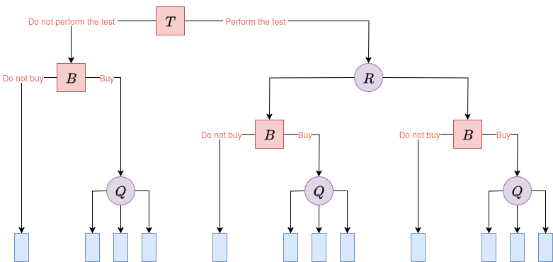
The number of decision paths is profoundly affected by the order and meaning of the variables (i.e., the problem’s definition). In our original oil field decision problem from Part I, the options Do not perform test and Do not buy prune the tree, resulting in 12 distinct decision paths. This is an asymmetric problem structure:
|
|
| Figure 1. Decision tree diagram of the asymmetric oil field investment problem from Part I. | |
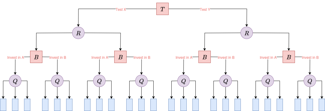
Conversely, a problem with the same types of variables, but structured symmetrically, would yield significantly more paths. For example, suppose the company must always begin by performing one of two possible geological tests (such as Test X or Test Y, each with different costs and accuracy profiles) on the field. Based on the test result, the company then chooses whether to Invest in Field A or Invest in Field B. After the investment decision, drilling reveals the field’s quality. This structure forces every path to be fully explored, doubling the number of distinct paths from 12 to 24:
|
|
| Figure 2. Decision tree diagram of a hypothetical symmetric oil field investment problem. | |
Even this revised example demonstrates how swiftly a decision tree can escalate beyond practical use. For instance, merely replacing the three-level oil quality (high/medium/low) with a more granular five-level scale (excellent/good/average/poor/dry) would push the total from 24 to 40 terminal nodes. This occurs without even considering longer time horizons, dynamic market-price scenarios, or additional complex choices.
This combinatorial explosion not only affects computational tractability but, even at more modest levels, severely compromises interpretability. As a rule of thumb, once a tree approaches about 100 terminal nodes, it loses its key strength: easy readability and intuitive understanding.
Hidden Conditional Independencies
In addition to the issue of combinatorial explosion, decision trees have another important limitation: they assume a strict, linear chain of dependence. In a decision tree, every variable is implicitly conditioned on all previous events along its particular path. This rigid structure prevents us from explicitly representing one of the most important concepts in probabilistic modeling: conditional independence.
To illustrate this, consider a generic problem with four random variables: \(\textcolor{purple}{A}\) and \(\textcolor{purple}{B}\) (each with two possible states, \(\textcolor{purple}{a_1}, \textcolor{purple}{a_2}\) and \(\textcolor{purple}{b_1}, \textcolor{purple}{b_2}\), respectively), and \(\textcolor{purple}{C}\) and \(\textcolor{purple}{D}\) (each with three possible states, \(\textcolor{purple}{c_1}, \textcolor{purple}{c_2}, \textcolor{purple}{c_3}\) and \(\textcolor{purple}{d_1}, \textcolor{purple}{d_2}, \textcolor{purple}{d_3}\)). In a traditional decision tree, where conditional independencies cannot be explicitly represented, you must specify the entire joint probability distribution for all variables. This means assigning a probability to every possible combination of outcomes, as shown in the joint probability table below:
P(A, B, C, D)
| $$\textcolor{purple}{A}$$ | $$\textcolor{purple}{B}$$ | $$\textcolor{purple}{C}$$ | $$\textcolor{purple}{D}$$ | Probability |
|---|---|---|---|---|
| $$\textcolor{purple}{a_{1}}$$ | $$\textcolor{purple}{b_{1}}$$ | $$\textcolor{purple}{c_{1}}$$ | $$\textcolor{purple}{d_{1}}$$ | $$P(\textcolor{purple}{a_{1}},\textcolor{purple}{b_{1}},\textcolor{purple}{c_{1}},\textcolor{purple}{d_{1}})$$ |
| $$\textcolor{purple}{a_{1}}$$ | $$\textcolor{purple}{b_{1}}$$ | $$\textcolor{purple}{c_{1}}$$ | $$\textcolor{purple}{d_{2}}$$ | $$P(\textcolor{purple}{a_{1}},\textcolor{purple}{b_{1}},\textcolor{purple}{c_{1}},\textcolor{purple}{d_{2}})$$ |
| $$\textcolor{purple}{a_{1}}$$ | $$\textcolor{purple}{b_{1}}$$ | $$\textcolor{purple}{c_{1}}$$ | $$\textcolor{purple}{d_{3}}$$ | $$P(\textcolor{purple}{a_{1}},\textcolor{purple}{b_{1}},\textcolor{purple}{c_{1}},\textcolor{purple}{d_{3}})$$ |
| $$\textcolor{purple}{a_{1}}$$ | $$\textcolor{purple}{b_{1}}$$ | $$\textcolor{purple}{c_{2}}$$ | $$\textcolor{purple}{d_{1}}$$ | $$P(\textcolor{purple}{a_{1}},\textcolor{purple}{b_{1}},\textcolor{purple}{c_{2}},\textcolor{purple}{d_{1}})$$ |
| $$\textcolor{purple}{a_{1}}$$ | $$\textcolor{purple}{b_{1}}$$ | $$\textcolor{purple}{c_{2}}$$ | $$\textcolor{purple}{d_{2}}$$ | $$P(\textcolor{purple}{a_{1}},\textcolor{purple}{b_{1}},\textcolor{purple}{c_{2}},\textcolor{purple}{d_{2}})$$ |
| $$\textcolor{purple}{a_{1}}$$ | $$\textcolor{purple}{b_{1}}$$ | $$\textcolor{purple}{c_{2}}$$ | $$\textcolor{purple}{d_{3}}$$ | $$P(\textcolor{purple}{a_{1}},\textcolor{purple}{b_{1}},\textcolor{purple}{c_{2}},\textcolor{purple}{d_{3}})$$ |
| $$\textcolor{purple}{a_{1}}$$ | $$\textcolor{purple}{b_{1}}$$ | $$\textcolor{purple}{c_{3}}$$ | $$\textcolor{purple}{d_{1}}$$ | $$P(\textcolor{purple}{a_{1}},\textcolor{purple}{b_{1}},\textcolor{purple}{c_{3}},\textcolor{purple}{d_{1}})$$ |
| $$\textcolor{purple}{a_{1}}$$ | $$\textcolor{purple}{b_{1}}$$ | $$\textcolor{purple}{c_{3}}$$ | $$\textcolor{purple}{d_{2}}$$ | $$P(\textcolor{purple}{a_{1}},\textcolor{purple}{b_{1}},\textcolor{purple}{c_{3}},\textcolor{purple}{d_{2}})$$ |
| $$\textcolor{purple}{a_{1}}$$ | $$\textcolor{purple}{b_{1}}$$ | $$\textcolor{purple}{c_{3}}$$ | $$\textcolor{purple}{d_{3}}$$ | $$P(\textcolor{purple}{a_{1}},\textcolor{purple}{b_{1}},\textcolor{purple}{c_{3}},\textcolor{purple}{d_{3}})$$ |
| $$\textcolor{purple}{a_{1}}$$ | $$\textcolor{purple}{b_{2}}$$ | $$\textcolor{purple}{c_{1}}$$ | $$\textcolor{purple}{d_{1}}$$ | $$P(\textcolor{purple}{a_{1}},\textcolor{purple}{b_{2}},\textcolor{purple}{c_{1}},\textcolor{purple}{d_{1}})$$ |
| $$\textcolor{purple}{a_{1}}$$ | $$\textcolor{purple}{b_{2}}$$ | $$\textcolor{purple}{c_{1}}$$ | $$\textcolor{purple}{d_{2}}$$ | $$P(\textcolor{purple}{a_{1}},\textcolor{purple}{b_{2}},\textcolor{purple}{c_{1}},\textcolor{purple}{d_{2}})$$ |
| $$\textcolor{purple}{a_{1}}$$ | $$\textcolor{purple}{b_{2}}$$ | $$\textcolor{purple}{c_{1}}$$ | $$\textcolor{purple}{d_{3}}$$ | $$P(\textcolor{purple}{a_{1}},\textcolor{purple}{b_{2}},\textcolor{purple}{c_{1}},\textcolor{purple}{d_{3}})$$ |
| $$\textcolor{purple}{a_{1}}$$ | $$\textcolor{purple}{b_{2}}$$ | $$\textcolor{purple}{c_{2}}$$ | $$\textcolor{purple}{d_{1}}$$ | $$P(\textcolor{purple}{a_{1}},\textcolor{purple}{b_{2}},\textcolor{purple}{c_{2}},\textcolor{purple}{d_{1}})$$ |
| $$\textcolor{purple}{a_{1}}$$ | $$\textcolor{purple}{b_{2}}$$ | $$\textcolor{purple}{c_{2}}$$ | $$\textcolor{purple}{d_{2}}$$ | $$P(\textcolor{purple}{a_{1}},\textcolor{purple}{b_{2}},\textcolor{purple}{c_{2}},\textcolor{purple}{d_{2}})$$ |
| $$\textcolor{purple}{a_{1}}$$ | $$\textcolor{purple}{b_{2}}$$ | $$\textcolor{purple}{c_{2}}$$ | $$\textcolor{purple}{d_{3}}$$ | $$P(\textcolor{purple}{a_{1}},\textcolor{purple}{b_{2}},\textcolor{purple}{c_{2}},\textcolor{purple}{d_{3}})$$ |
| $$\textcolor{purple}{a_{1}}$$ | $$\textcolor{purple}{b_{2}}$$ | $$\textcolor{purple}{c_{3}}$$ | $$\textcolor{purple}{d_{1}}$$ | $$P(\textcolor{purple}{a_{1}},\textcolor{purple}{b_{2}},\textcolor{purple}{c_{3}},\textcolor{purple}{d_{1}})$$ |
| $$\textcolor{purple}{a_{1}}$$ | $$\textcolor{purple}{b_{2}}$$ | $$\textcolor{purple}{c_{3}}$$ | $$\textcolor{purple}{d_{2}}$$ | $$P(\textcolor{purple}{a_{1}},\textcolor{purple}{b_{2}},\textcolor{purple}{c_{3}},\textcolor{purple}{d_{2}})$$ |
| $$\textcolor{purple}{a_{1}}$$ | $$\textcolor{purple}{b_{2}}$$ | $$\textcolor{purple}{c_{3}}$$ | $$\textcolor{purple}{d_{3}}$$ | $$P(\textcolor{purple}{a_{1}},\textcolor{purple}{b_{2}},\textcolor{purple}{c_{3}},\textcolor{purple}{d_{3}})$$ |
| $$\textcolor{purple}{a_{2}}$$ | $$\textcolor{purple}{b_{1}}$$ | $$\textcolor{purple}{c_{1}}$$ | $$\textcolor{purple}{d_{1}}$$ | $$P(\textcolor{purple}{a_{2}},\textcolor{purple}{b_{1}},\textcolor{purple}{c_{1}},\textcolor{purple}{d_{1}})$$ |
| $$\textcolor{purple}{a_{2}}$$ | $$\textcolor{purple}{b_{1}}$$ | $$\textcolor{purple}{c_{1}}$$ | $$\textcolor{purple}{d_{2}}$$ | $$P(\textcolor{purple}{a_{2}},\textcolor{purple}{b_{1}},\textcolor{purple}{c_{1}},\textcolor{purple}{d_{2}})$$ |
| $$\textcolor{purple}{a_{2}}$$ | $$\textcolor{purple}{b_{1}}$$ | $$\textcolor{purple}{c_{1}}$$ | $$\textcolor{purple}{d_{3}}$$ | $$P(\textcolor{purple}{a_{2}},\textcolor{purple}{b_{1}},\textcolor{purple}{c_{1}},\textcolor{purple}{d_{3}})$$ |
| $$\textcolor{purple}{a_{2}}$$ | $$\textcolor{purple}{b_{1}}$$ | $$\textcolor{purple}{c_{2}}$$ | $$\textcolor{purple}{d_{1}}$$ | $$P(\textcolor{purple}{a_{2}},\textcolor{purple}{b_{1}},\textcolor{purple}{c_{2}},\textcolor{purple}{d_{1}})$$ |
| $$\textcolor{purple}{a_{2}}$$ | $$\textcolor{purple}{b_{1}}$$ | $$\textcolor{purple}{c_{2}}$$ | $$\textcolor{purple}{d_{2}}$$ | $$P(\textcolor{purple}{a_{2}},\textcolor{purple}{b_{1}},\textcolor{purple}{c_{2}},\textcolor{purple}{d_{2}})$$ |
| $$\textcolor{purple}{a_{2}}$$ | $$\textcolor{purple}{b_{1}}$$ | $$\textcolor{purple}{c_{2}}$$ | $$\textcolor{purple}{d_{3}}$$ | $$P(\textcolor{purple}{a_{2}},\textcolor{purple}{b_{1}},\textcolor{purple}{c_{2}},\textcolor{purple}{d_{3}})$$ |
| $$\textcolor{purple}{a_{2}}$$ | $$\textcolor{purple}{b_{1}}$$ | $$\textcolor{purple}{c_{3}}$$ | $$\textcolor{purple}{d_{1}}$$ | $$P(\textcolor{purple}{a_{2}},\textcolor{purple}{b_{1}},\textcolor{purple}{c_{3}},\textcolor{purple}{d_{1}})$$ |
| $$\textcolor{purple}{a_{2}}$$ | $$\textcolor{purple}{b_{1}}$$ | $$\textcolor{purple}{c_{3}}$$ | $$\textcolor{purple}{d_{2}}$$ | $$P(\textcolor{purple}{a_{2}},\textcolor{purple}{b_{1}},\textcolor{purple}{c_{3}},\textcolor{purple}{d_{2}})$$ |
| $$\textcolor{purple}{a_{2}}$$ | $$\textcolor{purple}{b_{1}}$$ | $$\textcolor{purple}{c_{3}}$$ | $$\textcolor{purple}{d_{3}}$$ | $$P(\textcolor{purple}{a_{2}},\textcolor{purple}{b_{1}},\textcolor{purple}{c_{3}},\textcolor{purple}{d_{3}})$$ |
| $$\textcolor{purple}{a_{2}}$$ | $$\textcolor{purple}{b_{2}}$$ | $$\textcolor{purple}{c_{1}}$$ | $$\textcolor{purple}{d_{1}}$$ | $$P(\textcolor{purple}{a_{2}},\textcolor{purple}{b_{2}},\textcolor{purple}{c_{1}},\textcolor{purple}{d_{1}})$$ |
| $$\textcolor{purple}{a_{2}}$$ | $$\textcolor{purple}{b_{2}}$$ | $$\textcolor{purple}{c_{1}}$$ | $$\textcolor{purple}{d_{2}}$$ | $$P(\textcolor{purple}{a_{2}},\textcolor{purple}{b_{2}},\textcolor{purple}{c_{1}},\textcolor{purple}{d_{2}})$$ |
| $$\textcolor{purple}{a_{2}}$$ | $$\textcolor{purple}{b_{2}}$$ | $$\textcolor{purple}{c_{1}}$$ | $$\textcolor{purple}{d_{3}}$$ | $$P(\textcolor{purple}{a_{2}},\textcolor{purple}{b_{2}},\textcolor{purple}{c_{1}},\textcolor{purple}{d_{3}})$$ |
| $$\textcolor{purple}{a_{2}}$$ | $$\textcolor{purple}{b_{2}}$$ | $$\textcolor{purple}{c_{2}}$$ | $$\textcolor{purple}{d_{1}}$$ | $$P(\textcolor{purple}{a_{2}},\textcolor{purple}{b_{2}},\textcolor{purple}{c_{2}},\textcolor{purple}{d_{1}})$$ |
| $$\textcolor{purple}{a_{2}}$$ | $$\textcolor{purple}{b_{2}}$$ | $$\textcolor{purple}{c_{2}}$$ | $$\textcolor{purple}{d_{2}}$$ | $$P(\textcolor{purple}{a_{2}},\textcolor{purple}{b_{2}},\textcolor{purple}{c_{2}},\textcolor{purple}{d_{2}})$$ |
| $$\textcolor{purple}{a_{2}}$$ | $$\textcolor{purple}{b_{2}}$$ | $$\textcolor{purple}{c_{2}}$$ | $$\textcolor{purple}{d_{3}}$$ | $$P(\textcolor{purple}{a_{2}},\textcolor{purple}{b_{2}},\textcolor{purple}{c_{2}},\textcolor{purple}{d_{3}})$$ |
| $$\textcolor{purple}{a_{2}}$$ | $$\textcolor{purple}{b_{2}}$$ | $$\textcolor{purple}{c_{3}}$$ | $$\textcolor{purple}{d_{1}}$$ | $$P(\textcolor{purple}{a_{2}},\textcolor{purple}{b_{2}},\textcolor{purple}{c_{3}},\textcolor{purple}{d_{1}})$$ |
| $$\textcolor{purple}{a_{2}}$$ | $$\textcolor{purple}{b_{2}}$$ | $$\textcolor{purple}{c_{3}}$$ | $$\textcolor{purple}{d_{2}}$$ | $$P(\textcolor{purple}{a_{2}},\textcolor{purple}{b_{2}},\textcolor{purple}{c_{3}},\textcolor{purple}{d_{2}})$$ |
| $$\textcolor{purple}{a_{2}}$$ | $$\textcolor{purple}{b_{2}}$$ | $$\textcolor{purple}{c_{3}}$$ | $$\textcolor{purple}{d_{3}}$$ | $$P(\textcolor{purple}{a_{2}},\textcolor{purple}{b_{2}},\textcolor{purple}{c_{3}},\textcolor{purple}{d_{3}})$$ |
Total distinct probabilities: \(2 \; (\text{for } \textcolor{purple}{A}) \cdot 2 \; (\text{for } \textcolor{purple}{B}) \cdot 3 \; (\text{for } \textcolor{purple}{C}) \cdot 3 \; (\text{for } \textcolor{purple}{D}) = \mathbf{36}\).
Now, let’s say that conditional independencies do exist in this problem. For instance, let’s say that \(\textcolor{purple}{B}\) is conditionally independent of \(\textcolor{purple}{C}\) and \(\textcolor{purple}{D}\) given \(\textcolor{purple}{A}\). We denote that statement by \((\textcolor{purple}{B} \bot \{\textcolor{purple}{C}, \textcolor{purple}{D}\} \mid \textcolor{purple}{A})\). In that case:
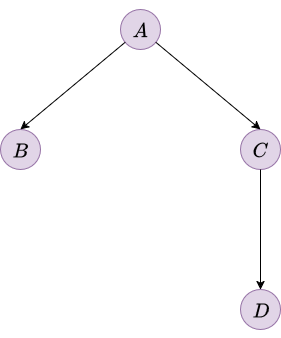
\[P(\textcolor{purple}{B} \mid \textcolor{purple}{A}, \textcolor{purple}{C}, \textcolor{purple}{D}) = P(\textcolor{purple}{B} \mid \textcolor{purple}{A})\]This fundamental concept allows us to represent relationships far more efficiently. Consider Figure 3, which implies the following conditional independence statements:
- \((\textcolor{purple}{B} \bot \{\textcolor{purple}{C}, \textcolor{purple}{D}\} \mid \textcolor{purple}{A})\)
- \((\textcolor{purple}{C} \bot \textcolor{purple}{B} \mid \textcolor{purple}{A})\)
- \((\textcolor{purple}{D} \bot \{\textcolor{purple}{A},\textcolor{purple}{B}\} \mid \textcolor{purple}{C})\)
The diagram corresponds to the directed acyclic graph of a Bayesian network, which visually encodes these independencies: arrows indicate direct probabilistic influence, while the absence of an arrow between two nodes reflects a conditional independence given their parents.
|
|
| Figure 3. Bayesian network illustrating conditional independencies among A, B, C, and D. | |
When these conditional independencies are recognized and modeled, we no longer need to construct a single large joint probability table. Instead, the full joint probability distribution can be factored into a product of smaller, more manageable conditional probability tables (CPTs). In our example, this means we only need to specify:
- \(P(\textcolor{purple}{A}) \rightarrow 2 = 2\) entries
- \(P(\textcolor{purple}{B} \mid \textcolor{purple}{A}) \rightarrow 2 \cdot 2 = 4\) entries
- \(P(\textcolor{purple}{C} \mid \textcolor{purple}{A}) \rightarrow 2 \cdot 3 = 6\) entries
- \(P(\textcolor{purple}{D} \mid \textcolor{purple}{C}) \rightarrow 3 \cdot 3 = 9\) entries
P(A)
| $$\textcolor{purple}{A}$$ | Probability |
|---|---|
| $$\textcolor{purple}{a_{1}}$$ | $$P(\textcolor{purple}{a_{1}})$$ |
| $$\textcolor{purple}{a_{2}}$$ | $$P(\textcolor{purple}{a_{2}})$$ |
P(B | A)
| $$\textcolor{purple}{A}$$ | $$\textcolor{purple}{B}$$ | Probability |
|---|---|---|
| $$\textcolor{purple}{a_{1}}$$ | $$\textcolor{purple}{b_{1}}$$ | $$P(\textcolor{purple}{b_{1}} \mid \textcolor{purple}{a_{1}})$$ |
| $$\textcolor{purple}{a_{1}}$$ | $$\textcolor{purple}{b_{2}}$$ | $$P(\textcolor{purple}{b_{2}} \mid \textcolor{purple}{a_{1}})$$ |
| $$\textcolor{purple}{a_{2}}$$ | $$\textcolor{purple}{b_{1}}$$ | $$P(\textcolor{purple}{b_{1}} \mid \textcolor{purple}{a_{2}})$$ |
| $$\textcolor{purple}{a_{2}}$$ | $$\textcolor{purple}{b_{2}}$$ | $$P(\textcolor{purple}{b_{2}} \mid \textcolor{purple}{a_{2}})$$ |
P(C | A)
| $$\textcolor{purple}{A}$$ | $$\textcolor{purple}{C}$$ | Probability |
|---|---|---|
| $$\textcolor{purple}{a_{1}}$$ | $$\textcolor{purple}{c_{1}}$$ | $$P(\textcolor{purple}{c_{1}} \mid \textcolor{purple}{a_{1}})$$ |
| $$\textcolor{purple}{a_{1}}$$ | $$\textcolor{purple}{c_{2}}$$ | $$P(\textcolor{purple}{c_{2}} \mid \textcolor{purple}{a_{1}})$$ |
| $$\textcolor{purple}{a_{1}}$$ | $$\textcolor{purple}{c_{3}}$$ | $$P(\textcolor{purple}{c_{3}} \mid \textcolor{purple}{a_{1}})$$ |
| $$\textcolor{purple}{a_{2}}$$ | $$\textcolor{purple}{c_{1}}$$ | $$P(\textcolor{purple}{c_{1}} \mid \textcolor{purple}{a_{2}})$$ |
| $$\textcolor{purple}{a_{2}}$$ | $$\textcolor{purple}{c_{2}}$$ | $$P(\textcolor{purple}{c_{2}} \mid \textcolor{purple}{a_{2}})$$ |
| $$\textcolor{purple}{a_{2}}$$ | $$\textcolor{purple}{c_{3}}$$ | $$P(\textcolor{purple}{c_{3}} \mid \textcolor{purple}{a_{2}})$$ |
P(D | C)
| $$\textcolor{purple}{C}$$ | $$\textcolor{purple}{D}$$ | Probability |
|---|---|---|
| $$\textcolor{purple}{c_{1}}$$ | $$\textcolor{purple}{d_{1}}$$ | $$P(\textcolor{purple}{d_{1}} \mid \textcolor{purple}{c_{1}})$$ |
| $$\textcolor{purple}{c_{1}}$$ | $$\textcolor{purple}{d_{2}}$$ | $$P(\textcolor{purple}{d_{2}} \mid \textcolor{purple}{c_{1}})$$ |
| $$\textcolor{purple}{c_{1}}$$ | $$\textcolor{purple}{d_{3}}$$ | $$P(\textcolor{purple}{d_{3}} \mid \textcolor{purple}{c_{1}})$$ |
| $$\textcolor{purple}{c_{2}}$$ | $$\textcolor{purple}{d_{1}}$$ | $$P(\textcolor{purple}{d_{1}} \mid \textcolor{purple}{c_{2}})$$ |
| $$\textcolor{purple}{c_{2}}$$ | $$\textcolor{purple}{d_{2}}$$ | $$P(\textcolor{purple}{d_{2}} \mid \textcolor{purple}{c_{2}})$$ |
| $$\textcolor{purple}{c_{2}}$$ | $$\textcolor{purple}{d_{3}}$$ | $$P(\textcolor{purple}{d_{3}} \mid \textcolor{purple}{c_{2}})$$ |
| $$\textcolor{purple}{c_{3}}$$ | $$\textcolor{purple}{d_{1}}$$ | $$P(\textcolor{purple}{d_{1}} \mid \textcolor{purple}{c_{3}})$$ |
| $$\textcolor{purple}{c_{3}}$$ | $$\textcolor{purple}{d_{2}}$$ | $$P(\textcolor{purple}{d_{2}} \mid \textcolor{purple}{c_{3}})$$ |
| $$\textcolor{purple}{c_{3}}$$ | $$\textcolor{purple}{d_{3}}$$ | $$P(\textcolor{purple}{d_{3}} \mid \textcolor{purple}{c_{3}})$$ |
Total distinct probabilities: \(2 + 4 + 6 + 9 = \mathbf{21}\).
This represents a 42% decrease from the 36 entries required in the full joint probability table. By reducing the number of parameters that must be specified, the model becomes much more manageable, transparent, and easier to modify. As decision problems increase in complexity, the advantages of explicitly modeling conditional independencies grow even more significant.
Influence Diagrams
Building on the foundation of Bayesian networks, influence diagrams (Howard & Matheson, 1984), also known as decision networks, provide a powerful extension that seamlessly integrates decision-making into probabilistic models. Unlike decision trees, influence diagrams avoid combinatorial explosion by factorizing the joint probability distribution and naturally express conditional independencies through their graphical structure.
An influence diagram enhances a Bayesian network by adding two types of nodes:
- Decision nodes: Shown as squares, these represent points where the decision-maker chooses among available actions.
- Outcome nodes: Illustrated as diamonds, these indicate the resulting utilities or values associated with different decision paths.
Chance nodes (circles) function as in Bayesian networks; when they are categorical, they are described by CPTs.
In influence diagrams, arcs serve two main purposes: informational arcs (into decision nodes) indicate what information is available when a choice is made, while conditional arcs (into chance or utility nodes) represent probabilistic or functional dependencies on parent variables, showing which factors affect outcomes or payoffs, without implying causality or temporal order.
Modelling the Oil Field Decision Problem
Modeling takes place at multiple levels. Drawing the influence diagram, much like constructing a decision tree, represents the qualitative description of the problem (structural level). Next, quantitative information is incorporated (numerical level) to fully specify the model.
A key limitation of influence diagrams is that they are only designed to handle symmetric problems. When faced with an asymmetric problem, it is necessary to transform it into a symmetric one, typically by introducing artificial states (which may be unintuitive). This transformation increases the size and complexity of the model, resulting in greater computational demands.
In large and highly asymmetric problems, using these resources (artificial states, degenerate probabilities, and utilities) to convert them into an equivalent symmetric one is not straightforward. For more information on this topic, see Bielza & Shenoy (1999).
To model the oil field decision problem, we will use a standard influence diagram. To maintain problem symmetry, an extra state called no results should be added to the porosity test results variable (R), since results are only observed when the test is performed.
Modelling Qualitative Information
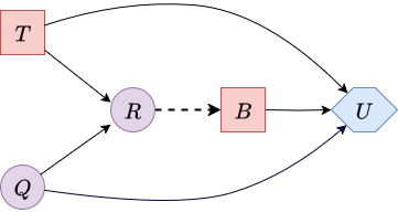
The following image displays the influence diagram structure for the decision problem:
|
|
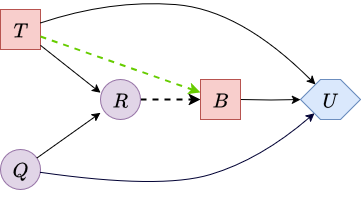
| Figure 4. Influence diagram for the oil field decision problem. Informational arcs are displayed with dashes. | |
This diagram illustrates a traditional influence diagram, which operates under the assumption of perfect recall. The information arcs indicate that the Test / No Test (\(\textcolor{red}{T}\)) decision is made prior to the Buy / No Buy (\(\textcolor{red}{B}\)) decision. Furthermore, no information is available before making the test decision, and the test results (\(\textcolor{purple}{R}\)) are known when making the buy decision. This establishes the temporal sequence of variables: \(\textcolor{red}{T}\), \(\textcolor{purple}{R}\), \(\textcolor{red}{B}\), and finally \(\textcolor{purple}{Q}\) (oil field quality).
However, traditional influence diagrams can become computationally complex to solve, particularly for intricate problems, and they may not accurately reflect the realistic limitations of human decision-making. For these reasons, LIMIDs (Lauritzen & Nilsson, 2001) are often the preferred choice. These models relax the perfect recall assumption and allow for explicit representation of limited memory. Memory arcs in LIMIDs explicitly specify which past decisions and observations are remembered and used for each current decision.
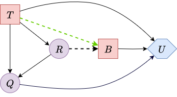
The subsequent image presents the corresponding LIMID, enhanced with a green memory arc. This memory arc extends from \(\textcolor{red}{T}\) to \(\textcolor{red}{B}\) because the outcome of the porosity test decision is crucial for the subsequent decision on buying or not buying the field.
|
|
| Figure 5. LIMID for the oil field decision problem with a memory arc shown in green. | |
Modelling Quantitative Information
Since all our random variables are categorical, we can conveniently represent the quantitative information of the model in tabular form. Below, we specify the prior probabilities, the CPTs, and the utility values relevant to the oil field decision problem.
Prior probabilities for the oil field quality (\(\textcolor{purple}{Q}\)):
| $$P(\textcolor{purple}{Q})$$ | |
|---|---|
| high | 0.35 |
| medium | 0.45 |
| low | 0.2 |
Conditional probabilities of observing each possible test result \(\textcolor{purple}{R}\), given the true oil field quality \(\textcolor{purple}{Q}\) and whether the test was performed \(\textcolor{red}{T}\):
| $$P(\textcolor{purple}{R} \mid \textcolor{purple}{Q},\, \textcolor{red}{T})$$ | perform | no perform | ||||
|---|---|---|---|---|---|---|
| high | medium | low | high | medium | low | |
| pass | 0.95 | 0.7 | 0.15 | 0 | 0 | 0 |
| fail | 0.05 | 0.3 | 0.85 | 0 | 0 | 0 |
| no results | 0 | 0 | 0 | 1 | 1 | 1 |
Utility (U) for each combination of test decision (T), buy decision (B), and oil field quality (Q):
| $$\textcolor{red}{T}$$ | $$\textcolor{red}{B}$$ | $$\textcolor{purple}{Q}$$ | $$\textcolor{blue}{U}$$ |
|---|---|---|---|
| perform | buy | high | 1220 |
| medium | 600 | ||
| low | -30 | ||
| no buy | high | 320 | |
| medium | 320 | ||
| low | 320 | ||
| no perform | buy | high | 1250 |
| medium | 630 | ||
| low | 0 | ||
| no buy | high | 350 | |
| medium | 350 | ||
| low | 350 |
Influence Diagram Evaluation
Influence diagrams were conceived as a compact, intuitive way to describe decision problems, yet practitioners initially had to transform them into a different format (i.e., a decision tree) in order to evaluate them. Until the 1980s, when Shachter (1986) showed how to evaluate the network directly, turning the diagram into a self-contained modelling and inference language.
Shachter’s arc-reversal / node-reduction algorithm reverses arcs and sequentially eliminates variables, summing over chance nodes and maximising over decision nodes while pushing expected-utility information forward.
Four Local Graph Operations
The arc-reversal / node-reduction algorithm employs a set of fundamental, local graph operations. Each operation ensures that the decision problem remains semantically equivalent, meaning the attainable utilities under any strategy are preserved:
-
Barren-Node Deletion: Any chance or decision node that has no children and is not a parent of an outcome node can be immediately removed from the diagram. Such nodes do not affect the utility and are therefore irrelevant to the decision problem.
Figure 6 illustrates the process of barren node elimination. The first diagram becomes the second, and then the third, since removing a barren node can create new barren nodes that can also be eliminated.

Figure 6. Barren node elimination example. -
Chance-Node Removal: Once a chance node \(\textcolor{purple}{C}\) becomes a leaf (i.e., it has no children except outcome nodes), it can be eliminated via marginalization (taking an expectation). For every outcome node \(\textcolor{blue}{O}\) that has \(\textcolor{purple}{C}\) as a parent, a new utility table, \(u'_{\textcolor{blue}{O}}\), is computed. This new table will depend on the original parents of \(\textcolor{blue}{O}\) (excluding \(\textcolor{purple}{C}\)) and all the parents of \(\textcolor{purple}{C}\).
\[u'_{\textcolor{blue}{O}}\left(\mathbf{\text{Pa}}_{\textcolor{blue}{O}} \cup \mathbf{\text{Pa}}_{\textcolor{purple}{C}} \setminus \{\textcolor{purple}{C}\}\right) = \sum_{\textcolor{purple}{c}} u_{\textcolor{blue}{O}}(\mathbf{\text{Pa}}_{\textcolor{blue}{O}}) \; P(\textcolor{purple}{c} \mid \mathbf{\text{Pa}}_{\textcolor{purple}{C}})\]Here:
- \(\mathbf{\text{Pa}}_{\textcolor{blue}{O}}\) denotes the set of parents of \(\textcolor{blue}{O}\) in the diagram before removing \(\textcolor{purple}{C}\).
- \(\mathbf{\text{Pa}}_{\textcolor{purple}{C}}\) denotes the set of parents of \(\textcolor{purple}{C}\).
- \(u'_{\textcolor{blue}{O}}\) represents the new utility table for node \(\textcolor{blue}{O}\).
Node \(\textcolor{purple}{C}\) and its CPT are then deleted. This operation “pushes expected utility forward” by embedding the influence of \(\textcolor{purple}{C}\) into the successor utility tables. The outcome node \(\textcolor{blue}{O}\) effectively inherits the predecessors of \(\textcolor{purple}{C}\), ensuring that all relevant dependencies are preserved.Figure 7 showcases the process of chance node removal, specifically \(\textcolor{purple}{C_2}\). The first diagram becomes the second, where parents of \(\textcolor{purple}{C_{2}}\) become the parents of \(\textcolor{blue}{O_1}\).
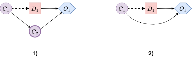
Figure 7. Chance node removal example. -
Decision-Node Removal: When a decision node \(\textcolor{red}{D}\) becomes a leaf in the influence diagram, meaning its only children are outcome nodes \(\textcolor{blue}{O}\), it can be eliminated. This step requires identifying the optimal decision for \(\textcolor{red}{D}\) in every possible situation, or “information state”, defined by the specific combination of observed values of \(\textcolor{red}{D}\)’s parent nodes.
For each information state \(i\), we choose the action \(\textcolor{red}{d}\) that maximizes the expected utility \(\mathbb{E}[u(\textcolor{red}{d}, i)]\). This action represents the best possible choice for that information state and forms part of the overall optimal policy:
\[\delta^*(i) = \text{argmax}_{\textcolor{red}{d}} \ \mathbb{E}[u(\textcolor{red}{d}, i)]\]The function \(\delta^*(i)\) is recorded as the optimal decision rule for node \(\textcolor{red}{D}\) in information state \(i\). After removing \(\textcolor{red}{D}\), each outcome node \(\textcolor{blue}{O}\) that was a child of \(\textcolor{red}{D}\) has its utility table updated to reflect the maximum expected utility (MEU) achievable by making the optimal decision at \(\textcolor{red}{D}\), given the information state \(i\).
This process “locks in” the optimal strategy for \(\textcolor{red}{D}\) and propagates the MEU forward through the diagram, similar to how chance nodes \(\textcolor{purple}{C}\) are eliminated by marginalization.
Figure 8 demonstrates the process of eliminating a decision node, specifically \(\textcolor{red}{D_2}\). In the first diagram, the decision node is present; in the second, it has been removed, and the utility table has been updated to incorporate the optimal decision rule \(\delta^*(\textcolor{red}{D_2})\) for each information state (i.e., each combination of parent values). Only the maximum attainable utilities for each state are preserved.
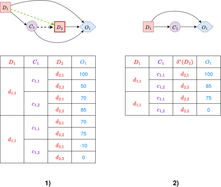
Figure 8. Decision node removal example. -
Arc Reversal (between chance nodes): In most influence diagrams, nodes are not naturally leaves. They may have children that prevent us from eliminating them directly. To solve this, we use arc reversal to make a target node into a leaf by pushing its influence “backwards” to its children and adjusting the rest of the diagram so that it still represents the same probabilistic relationships.
Let’s say we want to reverse an arc \(\textcolor{purple}{X} \rightarrow \textcolor{purple}{Y}\) where \(\mathbf{\text{Pa}}_{\textcolor{purple}{X}}\) is the set of parents of \(\textcolor{purple}{X}\) and \(\mathbf{\text{Pa}}_{\textcolor{purple}{Y}}\) is the parents of \(\textcolor{purple}{Y}\), including \(\textcolor{purple}{X}\) itself.
To reverse, we remove the arc \(\textcolor{purple}{X} \rightarrow \textcolor{purple}{Y}\), add a new arc \(\textcolor{purple}{Y} \rightarrow \textcolor{purple}{X}\), add arcs from \(\mathbf{\text{Pa}}_{\textcolor{purple}{X}}\) to \(\textcolor{purple}{Y}\) if they are not already parents of \(\textcolor{purple}{Y}\), and add arcs from \(\mathbf{\text{Pa}}_{\textcolor{purple}{Y}}\) to \(\textcolor{purple}{X}\), if needed, to preserve dependencies. This means the new parents of \(\textcolor{purple}{X}\) and \(\textcolor{purple}{Y}\) are:
- \(\mathbf{\text{Pa}}^{\text{new}}_{\textcolor{purple}{Y}} = \mathbf{\text{Pa}}_{\textcolor{purple}{X}} \cup \mathbf{\text{Pa}}_{\textcolor{purple}{Y}} \setminus \{\textcolor{purple}{Y}\}\)
- \(\mathbf{\text{Pa}}^{\text{new}}_{\textcolor{purple}{X}} = \mathbf{\text{Pa}}_{\textcolor{purple}{X}} \cup \mathbf{\text{Pa}}_{\textcolor{purple}{Y}} \cup \{\textcolor{purple}{Y}\} \setminus \{\textcolor{purple}{X}\}\)
\[\begin{aligned} P(\textcolor{purple}{Y} \mid \mathbf{\text{Pa}}^{\text{new}}_{\textcolor{purple}{Y}}) &= \sum_{\textcolor{purple}{X}} P(\textcolor{purple}{Y} \mid \mathbf{\text{Pa}}_{\textcolor{purple}{Y}}) \cdot P(\textcolor{purple}{X} \mid \mathbf{\text{Pa}}_{\textcolor{purple}{X}}) \\ \\ P(\textcolor{purple}{X} \mid \mathbf{\text{Pa}}^{\text{new}}_{\textcolor{purple}{X}}) &= \frac{P(\textcolor{purple}{Y} \mid \mathbf{\text{Pa}}_{\textcolor{purple}{Y}}) \cdot P(\textcolor{purple}{X} \mid \mathbf{\text{Pa}}_{\textcolor{purple}{X}})}{P(\textcolor{purple}{Y} \mid \mathbf{\text{Pa}}^{\text{new}}_{\textcolor{purple}{Y}})} \end{aligned}\]
To ensure the joint distribution remains unchanged under the new structure, we compute the new CPT using Bayes’ Theorem:As an example, consider the influence diagram shown in Figure 9, which contains three chance nodes. We will reverse the arc \(\textcolor{purple}{C_2} \rightarrow \textcolor{purple}{C_3}\). Before reversal, the parent sets are:
- \(\mathbf{\text{Pa}}_{\textcolor{purple}{C_2}} = \{\textcolor{purple}{C_1}\}\)
- \(\mathbf{\text{Pa}}_{\textcolor{purple}{C_3}} = \{\textcolor{purple}{C_2}\}\)
After reversal, the new parent sets become:
- \(\mathbf{\text{Pa}}^{\text{new}}_{\textcolor{purple}{C_2}} = \{\textcolor{purple}{C_1}, \textcolor{purple}{C_3}\}\)
- \(\mathbf{\text{Pa}}^{\text{new}}_{\textcolor{purple}{C_3}} = \{\textcolor{purple}{C_1}\}\)
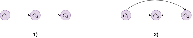
Figure 9. Arc reversal example. We are given the following initial CPTs:
$$P(\textcolor{purple}{C_1})$$ $$\textcolor{purple}{c_{1,1}}$$ 0.7 $$\textcolor{purple}{c_{1,2}}$$ 0.3 $$P(\textcolor{purple}{C_2} \mid \textcolor{purple}{C_1})$$ $$\textcolor{purple}{c_{1,1}}$$ $$\textcolor{purple}{c_{1,2}}$$ $$\textcolor{purple}{c_{2,1}}$$ 0.6 0.1 $$\textcolor{purple}{c_{2,2}}$$ 0.4 0.9 $$P(\textcolor{purple}{C_3} \mid \textcolor{purple}{C_2})$$ $$\textcolor{purple}{c_{2,1}}$$ $$\textcolor{purple}{c_{2,2}}$$ $$\textcolor{purple}{c_{3,1}}$$ 0.9 0.2 $$\textcolor{purple}{c_{3,2}}$$ 0.1 0.8 Step 1: Compute new CPT for \(P(\textcolor{purple}{C_3} \mid \textcolor{purple}{C_1})\)
Using marginalization:
\[P(\textcolor{purple}{C_3} \mid \textcolor{purple}{C_1}) = \sum_{\textcolor{purple}{c_2}} P(\textcolor{purple}{C_3} \mid \textcolor{purple}{c_2}) P(\textcolor{purple}{c_2} \mid \textcolor{purple}{C_1}).\]\(\textcolor{purple}{c_{1,1}}\):
\[\begin{aligned} P(\textcolor{purple}{c_{3,1}} \mid \textcolor{purple}{c_{1,1}}) &= P(\textcolor{purple}{c_{3,1}} \mid \textcolor{purple}{c_{2,2}})P(\textcolor{purple}{c_{2,2}} \mid \textcolor{purple}{c_{1,1}}) + P(\textcolor{purple}{c_{3,1}} \mid \textcolor{purple}{c_{2,1}})P(\textcolor{purple}{c_{2,1}} \mid \textcolor{purple}{c_{1,1}}) \\ &= 0.2 \cdot 0.4 + 0.9 \cdot 0.6 \\ &= 0.08 + 0.54 = 0.62 \\ P(\textcolor{purple}{c_{3,2}} \mid \textcolor{purple}{c_{1,1}}) &= 1 - P(\textcolor{purple}{c_{3,1}} \mid \textcolor{purple}{c_{1,1}}) = 1 - 0.62 = 0.38 \end{aligned}\]\(\textcolor{purple}{c_{1,2}}\):
\[\begin{aligned} P(\textcolor{purple}{c_{3,1}} \mid \textcolor{purple}{c_{1,2}}) &= P(\textcolor{purple}{c_{3,1}} \mid \textcolor{purple}{c_{2,2}})P(\textcolor{purple}{c_{2,2}} \mid \textcolor{purple}{c_{1,2}}) + P(\textcolor{purple}{c_{3,1}} \mid \textcolor{purple}{c_{2,1}})P(\textcolor{purple}{c_{2,1}} \mid \textcolor{purple}{c_{1,2}}) \\ &= 0.2 \cdot 0.9 + 0.9 \cdot 0.1 \\ &= 0.18 + 0.09 = 0.27 \\ P(\textcolor{purple}{c_{3,2}} \mid \textcolor{purple}{c_{1,2}}) &= 1 - P(\textcolor{purple}{c_{3,1}} \mid \textcolor{purple}{c_{1,2}}) = 1 - 0.27 = 0.73 \end{aligned}\]Summarized as:
$$P(\textcolor{purple}{C_3} \mid \textcolor{purple}{C_1})$$ $$\textcolor{purple}{c_{1,1}}$$ $$\textcolor{purple}{c_{1,2}}$$ $$\textcolor{purple}{c_{3,1}}$$ 0.62 0.27 $$\textcolor{purple}{c_{3,2}}$$ 0.38 0.73 Step 2: Compute new CPT for \(P(\textcolor{purple}{C_2} \mid \textcolor{purple}{C_1}, \textcolor{purple}{C_3})\)
Using Bayes’ Theorem, rounding results to three decimal places:
\[P(\textcolor{purple}{C_2} \mid \textcolor{purple}{C_1}, \textcolor{purple}{C_3}) = \frac{P(\textcolor{purple}{C_3} \mid \textcolor{purple}{C_2}) \, P(\textcolor{purple}{C_2} \mid \textcolor{purple}{C_1})}{P(\textcolor{purple}{C_3} \mid \textcolor{purple}{C_1})}.\](\(\textcolor{purple}{c_{1,1}}\), \(\textcolor{purple}{c_{3,1}}\)):
\[\begin{aligned} &\quad P(\textcolor{purple}{c_{2,1}} \mid \textcolor{purple}{c_{1,1}}, \textcolor{purple}{c_{3,1}}) = \frac{P(\textcolor{purple}{c_{3,1}} \mid \textcolor{purple}{c_{2,1}}) \, P(\textcolor{purple}{c_{2,1}} \mid \textcolor{purple}{c_{1,1}})}{P(\textcolor{purple}{c_{3,1}} \mid \textcolor{purple}{c_{1,1}})} = \frac{0.9 \cdot 0.6}{0.62} = 0.871 \\ &\quad P(\textcolor{purple}{c_{2,2}} \mid \textcolor{purple}{c_{1,1}}, \textcolor{purple}{c_{3,1}}) = 1 - P(\textcolor{purple}{c_{2,1}} \mid \textcolor{purple}{c_{1,1}}, \textcolor{purple}{c_{3,1}}) = 1 - 0.871 = 0.129 \end{aligned}\](\(\textcolor{purple}{c_{1,2}}\), \(\textcolor{purple}{c_{3,1}}\)):
\[\begin{aligned} &\quad P(\textcolor{purple}{c_{2,1}} \mid \textcolor{purple}{c_{1,2}}, \textcolor{purple}{c_{3,1}}) = \frac{P(\textcolor{purple}{c_{3,1}} \mid \textcolor{purple}{c_{2,1}}) \, P(\textcolor{purple}{c_{2,1}} \mid \textcolor{purple}{c_{1,2}})}{P(\textcolor{purple}{c_{3,1}} \mid \textcolor{purple}{c_{1,2}})} = \frac{0.9 \cdot 0.1}{0.27} = 0.333 \\ &\quad P(\textcolor{purple}{c_{2,2}} \mid \textcolor{purple}{c_{1,2}}, \textcolor{purple}{c_{3,1}}) = 1 - P(\textcolor{purple}{c_{2,1}} \mid \textcolor{purple}{c_{1,2}}, \textcolor{purple}{c_{3,1}}) = 1 - 0.333 = 0.667 \\[3ex] \end{aligned}\](\(\textcolor{purple}{c_{1,1}}\), \(\textcolor{purple}{c_{3,2}}\)):
\[\begin{aligned} &\quad P(\textcolor{purple}{c_{2,1}} \mid \textcolor{purple}{c_{1,1}}, \textcolor{purple}{c_{3,2}}) = \frac{P(\textcolor{purple}{c_{3,2}} \mid \textcolor{purple}{c_{2,1}}) \, P(\textcolor{purple}{c_{2,1}} \mid \textcolor{purple}{c_{1,1}})}{P(\textcolor{purple}{c_{3,2}} \mid \textcolor{purple}{c_{1,1}})} = \frac{0.1 \cdot 0.6}{0.38} = 0.158 \\ &\quad P(\textcolor{purple}{c_{2,2}} \mid \textcolor{purple}{c_{1,1}}, \textcolor{purple}{c_{3,2}}) = 1 - P(\textcolor{purple}{c_{2,1}} \mid \textcolor{purple}{c_{1,1}}, \textcolor{purple}{c_{3,2}}) = 1 - 0.158 = 0.842 \\[3ex] \end{aligned}\](\(\textcolor{purple}{c_{1,2}}\), \(\textcolor{purple}{c_{3,2}}\)):
\[\begin{aligned} &\quad P(\textcolor{purple}{c_{2,1}} \mid \textcolor{purple}{c_{1,2}}, \textcolor{purple}{c_{3,2}}) = \frac{P(\textcolor{purple}{c_{3,2}} \mid \textcolor{purple}{c_{2,1}}) \, P(\textcolor{purple}{c_{2,1}} \mid \textcolor{purple}{c_{1,2}})}{P(\textcolor{purple}{c_{3,2}} \mid \textcolor{purple}{c_{1,2}})} = \frac{0.1 \cdot 0.1}{0.73} = 0.014 \\ &\quad P(\textcolor{purple}{c_{2,2}} \mid \textcolor{purple}{c_{1,2}}, \textcolor{purple}{c_{3,2}}) = 1 - P(\textcolor{purple}{c_{2,1}} \mid \textcolor{purple}{c_{1,2}}, \textcolor{purple}{c_{3,2}}) = 1 - 0.014 = 0.986 \\[3ex] \end{aligned}\]Summarized as:
$$P(\textcolor{purple}{C_2} \mid \textcolor{purple}{C_1}, \textcolor{purple}{C_3})$$ $$\textcolor{purple}{c_{3,1}}$$ $$\textcolor{purple}{c_{3,2}}$$ $$\textcolor{purple}{c_{1,1}}$$ $$\textcolor{purple}{c_{1,2}}$$ $$\textcolor{purple}{c_{1,1}}$$ $$\textcolor{purple}{c_{1,2}}$$ $$\textcolor{purple}{c_{2,1}}$$ 0.871 0.333 0.158 0.014 $$\textcolor{purple}{c_{2,2}}$$ 0.129 0.667 0.842 0.986
The Arc-Reversal / Node-Reduction Algorithm
The algorithm incrementally eliminates nodes by repeatedly applying the four local graph operations described above, until only a single value node remains. The number stored in this final value node is the MEU, and the collection of recorded decision rules forms an optimal policy for the original decision problem.
Input: A well-formed influence diagram (or LIMID).
Output: The MEU and an optimal policy for each decision node.
Preparatory steps:
- Canonical form: If the diagram does not already satisfy the standard conventions (total order of decisions, and no arcs from decisions to chance nodes), perform a sequence of Arc Reversals (Rule 4) to obtain a canonical influence diagram.
- LIMID transformation: Transform the influence diagram into a LIMID by adding memory arcs so that each decision node has, as parents, all information variables that are remembered at the time of the decision.
Main loop - repeat until only one value node remains:
- Select a node \(N\) to eliminate
- If there is any barren node (a node with no children), delete it immediately using Barren-Node Deletion (Rule 1).
- Otherwise, select any leaf node (a chance or decision node whose only children are value nodes).
- If no leaf exists, choose a non-value node and repeatedly apply Arc Reversal (Rule 4) to its outgoing arcs until it becomes a leaf.
- Eliminate \(N\)
- If \(N\) is a chance node, apply Chance-Node Removal (Rule 2): marginalize over \(N\) and update the relevant value tables.
- If \(N\) is a decision node, apply Decision-Node Removal (Rule 3): maximize over the possible actions of \(N\), record the optimal decision rule \(\delta^*\), and update the value tables.
- Merge any duplicate value nodes that may have arisen during elimination.
When the loop ends, only one value node remains. Its single numerical entry is the MEU. The set \(\{\delta^*\}\) collected during the process provides an optimal decision rule for each decision node.
Relationship to Bayesian Network Variable Elimination
Arc reversal/node reduction in influence diagrams is structurally similar to variable elimination in Bayesian networks. The main difference is the handling of utilities via maximization over decision nodes (instead of summation over chance nodes). In both approaches, information is propagated through the graph by combining local factors (such as CPTs or utility functions) and eliminating variables, either by summing over uncertainties for chance nodes or optimizing (maximizing) over decisions for decision nodes.
This similarity also extends to computational complexity: since both methods generate and manipulate similar intermediate factors, their efficiency is determined by the treewidth of the chosen elimination order.
Related Work
There are several alternative strategies for evaluating influence diagrams beyond the arc-reversal and node-reduction procedures described above.
A more compact exact method is junction-tree propagation, which is also inspired by techniques from Bayesian networks. In this approach, the influence diagram is first moralized and triangulated, then compiled into a tree of cliques. Local probability and utility factors are passed between cliques using message-passing algorithms such as Shafer-Shenoy (Shafer & Shenoy, 1990) or HUGIN until convergence is reached. Junction-tree algorithms are often more memory-efficient than straightforward variable elimination and form the foundation of many commercial and open-source tools, including PyAgrum (Jensen et al., 1994; Madsen & Jensen, 1999; Lauritzen & Nilsson, 2001).
However, even junction-tree propagation can become impractical for very complex or densely connected models, as the required clique tables may grow prohibitively large. Additionally, exact arc-reversal is difficult when the diagram contains continuous variables. In these situations, we need to rely on approximate methods. The most common of these is Monte Carlo sampling, which estimates expected utility by simulating random scenarios (Shachter & Kenley, 1989; Jenzarli, 1995). Later research has shown that Monte Carlo methods can be extended to handle non-Gaussian or hybrid influence diagrams (Bielza et al., 1999; Cobb & Shenoy, 2008).
Finally, another avenue is variational inference, although I haven’t yet found published work applying it to influence diagrams. In principle, one could adapt techniques such as variational message passing (Winn & Bishop, 2005) to do so.
Evaluating the Oil Influence Diagram
We will use the arc-reversal / node-reduction algorithm to solve the oil field decision problem. Note that the influence diagram is already a LIMID, since we added the arc \(\textcolor{red}{T} \rightarrow \textcolor{red}{B}\), and it is in canonical form.
In Figure 5, we observe that there are neither barren nodes nor leaf nodes. Therefore, we must select one of the chance nodes and apply arc reversal until it becomes a leaf.
For the first step, we select node \(\textcolor{purple}{Q}\) (oil field quality). Therefore, we need to reverse the arc \(\textcolor{purple}{Q} \rightarrow \textcolor{purple}{R}\). To do this, we remove the arc \(\textcolor{purple}{Q} \rightarrow \textcolor{purple}{R}\), add the arc \(\textcolor{purple}{R} \rightarrow \textcolor{purple}{Q}\), and add arcs from the parents of \(\textcolor{purple}{R}\) to \(\textcolor{purple}{Q}\) if they are not already parents of \(\textcolor{purple}{Q}\). This also means adding the arc \(\textcolor{red}{T} \rightarrow \textcolor{purple}{R}\).
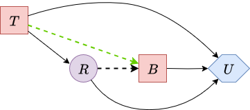
Figure 10 shows the result of reversing \(\textcolor{purple}{Q} \rightarrow \textcolor{purple}{R}\):
|
|
| Figure 10. Influence diagram after reversing arc Q → R. | |
To obtain the distribution \(P(\textcolor{purple}{R} \mid \textcolor{red}{T})\), we first marginalize over \(\textcolor{purple}{Q}\) in \(P(\textcolor{purple}{R} \mid \textcolor{purple}{Q})\):
Posteriors for pass and fail results
$$ \begin{aligned} P(\textcolor{purple}{\text{pass}} \mid \textcolor{purple}{Q}) &= P(\textcolor{purple}{\text{pass}} \mid \textcolor{purple}{\text{high}})P(\textcolor{purple}{\text{high}}) + P(\textcolor{purple}{\text{pass}} \mid \textcolor{purple}{\text{medium}})P(\textcolor{purple}{\text{medium}}) + P(\textcolor{purple}{\text{pass}} \mid \textcolor{purple}{\text{low}})P(\textcolor{purple}{\text{low}}) \\ &= 0.95 \cdot 0.35 + 0.7 \cdot 0.45 + 0.15 \cdot 0.2 \\ &= 0.3325 + 0.315 + 0.03 \\ &= 0.6775 \\[1em] P(\textcolor{purple}{\text{fail}} \mid \textcolor{purple}{Q}) &= P(\textcolor{purple}{\text{fail}} \mid \textcolor{purple}{\text{high}})P(\textcolor{purple}{\text{high}}) + P(\textcolor{purple}{\text{fail}} \mid \textcolor{purple}{\text{medium}})P(\textcolor{purple}{\text{medium}}) + P(\textcolor{purple}{\text{fail}} \mid \textcolor{purple}{\text{low}})P(\textcolor{purple}{\text{low}}) \\ &= 0.05 \cdot 0.35 + 0.3 \cdot 0.45 + 0.85 \cdot 0.2 \\ &= 0.0175 + 0.135 + 0.17 \\ &= 0.3225 \\ \end{aligned} $$Now, given that R only applies when we make the test, we know that \(P\left(\textcolor{purple}{R} \mid \textcolor{purple}{Q},\, \textcolor{red}{T} = \textcolor{red}{\text{perform}}\right)\) is simply \(P\left(\textcolor{purple}{R} \mid \textcolor{purple}{Q}\right)\), and that \(P\left(\textcolor{purple}{R} \mid \textcolor{purple}{Q},\, \textcolor{red}{T} = \textcolor{red}{\text{no perform}}\right)\) is all zeros except for the no results case. Therefore:
| $$P(\textcolor{purple}{R} \mid \textcolor{red}{T})$$ | perform | no perform |
|---|---|---|
| pass | 0.6775 | 0 |
| fail | 0.3225 | 0 |
| no results | 0 | 1 |
Now for \(P(\textcolor{purple}{Q} \mid \textcolor{purple}{R})\), we need to apply Bayes’ theorem:
P(Q | R = pass)
$$ \begin{aligned} P(\textcolor{purple}{\text{high}} \mid \textcolor{purple}{\text{pass}}) &= \frac{P(\textcolor{purple}{\text{pass}} \mid \textcolor{purple}{\text{high}})P(\textcolor{purple}{\text{high}})}{P(\textcolor{purple}{\text{pass}})} \\ &= \frac{0.95 \cdot 0.35}{0.6775} = \frac{0.3325}{0.6775} \approx 0.4908 \\[1em] P(\textcolor{purple}{\text{medium}} \mid \textcolor{purple}{\text{pass}}) &= \frac{P(\textcolor{purple}{\text{pass}} \mid \textcolor{purple}{\text{medium}})P(\textcolor{purple}{\text{medium}})}{P(\textcolor{purple}{\text{pass}})} \\ &= \frac{0.7 \cdot 0.45}{0.6775} = \frac{0.315}{0.6775} \approx 0.4649 \\[1em] P(\textcolor{purple}{\text{low}} \mid \textcolor{purple}{\text{pass}}) &= \frac{P(\textcolor{purple}{\text{pass}} \mid \textcolor{purple}{\text{low}})P(\textcolor{purple}{\text{low}})}{P(\textcolor{purple}{\text{pass}})} \\ &= \frac{0.15 \cdot 0.2}{0.6775} = \frac{0.03}{0.6775} \approx 0.0443 \end{aligned} $$P(Q | R = fail)
$$ \begin{aligned} P(\textcolor{purple}{\text{high}} \mid \textcolor{purple}{\text{fail}}) &= \frac{P(\textcolor{purple}{\text{fail}} \mid \textcolor{purple}{\text{high}})P(\textcolor{purple}{\text{high}})}{P(\textcolor{purple}{\text{fail}})} \\ &= \frac{0.05 \cdot 0.35}{0.3225} = \frac{0.0175}{0.3225} \approx 0.0543 \\[1em] P(\textcolor{purple}{\text{medium}} \mid \textcolor{purple}{\text{fail}}) &= \frac{P(\textcolor{purple}{\text{fail}} \mid \textcolor{purple}{\text{medium}})P(\textcolor{purple}{\text{medium}})}{P(\textcolor{purple}{\text{fail}})} \\ &= \frac{0.3 \cdot 0.45}{0.3225} = \frac{0.135}{0.3225} \approx 0.4186 \\[1em] P(\textcolor{purple}{\text{low}} \mid \textcolor{purple}{\text{fail}}) &= \frac{P(\textcolor{purple}{\text{fail}} \mid \textcolor{purple}{\text{low}})P(\textcolor{purple}{\text{low}})}{P(\textcolor{purple}{\text{fail}})} \\ &= \frac{0.85 \cdot 0.2}{0.3225} = \frac{0.17}{0.3225} \approx 0.5271 \end{aligned} $$When \(\textcolor{red}{T} = \textcolor{red}{\text{no perform}}\), then \(\textcolor{purple}{R}\) does not make sense, so \(P\left(\textcolor{purple}{Q} \mid \textcolor{purple}{R},\, \textcolor{red}{T} = \textcolor{red}{\text{no perform}}\right)\) is simply \(P\left(\textcolor{purple}{Q}\right)\). Therefore:
| $$P(\textcolor{purple}{Q} \mid \textcolor{purple}{R},\, \textcolor{red}{T})$$ | perform | no perform | ||||
|---|---|---|---|---|---|---|
| pass | fail | no results | pass | fail | no results | |
| high | 0.4908 | 0.0543 | x | x | x | 0.35 |
| medium | 0.4649 | 0.4186 | x | x | x | 0.45 |
| low | 0.0443 | 0.5271 | x | x | x | 0.2 |
By making the problem symmetric, we have introduced many zero probabilities, which increases the likelihood of encountering undefined expressions such as \(0/0\). Recall that a conditional probability \(P(\textcolor{purple}{a} \mid \textcolor{purple}{b})\) is only defined when \(P(\textcolor{purple}{b}) > 0\), so we should not expect to be able to compute every conditional probability when reversing arcs. However, as will be shown below, these “x” values will not affect the outcome of the problem.
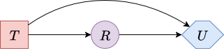
After reversing the arc \(\textcolor{purple}{Q} \rightarrow \textcolor{purple}{R}\), the node \(\textcolor{purple}{Q}\) becomes a leaf and can be eliminated. Figure 11 illustrates the resulting diagram.
|
|
| Figure 11. Influence diagram after removing node Q. | |
By removing \(\textcolor{purple}{Q}\), we need to marginalize it and update the utility table of \(\textcolor{blue}{U}\)
\[u'_\textcolor{blue}{U}(\textcolor{red}{T}, \textcolor{purple}{R}, \textcolor{red}{B}) = \sum_{\textcolor{purple}{q}} u_\textcolor{blue}{U}(\textcolor{red}{T}, \textcolor{red}{B}, \textcolor{purple}{Q})P(\textcolor{purple}{q} \mid \textcolor{red}{T}, \textcolor{purple}{R})\]U'(R, B, T = perform)
$$ \begin{aligned} u'_\textcolor{blue}{U}(\textcolor{red}{\text{perform}},\ \textcolor{purple}{\text{pass}},\ \textcolor{red}{\text{buy}}) &= u_\textcolor{blue}{U}(\textcolor{red}{\text{perform}}, \textcolor{red}{\text{buy}}, \textcolor{purple}{\text{high}}) P(\textcolor{purple}{\text{high}} \mid \textcolor{red}{\text{perform}}, \textcolor{purple}{\text{pass}}) \\ &\quad + u_\textcolor{blue}{U}(\textcolor{red}{\text{perform}}, \textcolor{red}{\text{buy}}, \textcolor{purple}{\text{medium}}) P(\textcolor{purple}{\text{medium}} \mid \textcolor{red}{\text{perform}}, \textcolor{purple}{\text{pass}}) \\ &\quad + u_\textcolor{blue}{U}(\textcolor{red}{\text{perform}}, \textcolor{red}{\text{buy}}, \textcolor{purple}{\text{low}}) P(\textcolor{purple}{\text{low}} \mid \textcolor{red}{\text{perform}}, \textcolor{purple}{\text{pass}}) \\ &= 1220 \cdot 0.4908 + 600 \cdot 0.4649 + (-30) \cdot 0.0443 \\ &= 598.776 + 278.94 - 1.329 \\ &= 876.387 \\[1em] % ------------------- u'_\textcolor{blue}{U}(\textcolor{red}{\text{perform}},\ \textcolor{purple}{\text{pass}},\ \textcolor{red}{\text{no buy}}) &= u_\textcolor{blue}{U}(\textcolor{red}{\text{perform}}, \textcolor{red}{\text{no buy}}, \textcolor{purple}{\text{high}}) P(\textcolor{purple}{\text{high}} \mid \textcolor{red}{\text{perform}}, \textcolor{purple}{\text{pass}}) \\ &\quad + u_\textcolor{blue}{U}(\textcolor{red}{\text{perform}}, \textcolor{red}{\text{no buy}}, \textcolor{purple}{\text{medium}}) P(\textcolor{purple}{\text{medium}} \mid \textcolor{red}{\text{perform}}, \textcolor{purple}{\text{pass}}) \\ &\quad + u_\textcolor{blue}{U}(\textcolor{red}{\text{perform}}, \textcolor{red}{\text{no buy}}, \textcolor{purple}{\text{low}}) P(\textcolor{purple}{\text{low}} \mid \textcolor{red}{\text{perform}}, \textcolor{purple}{\text{pass}}) \\ &= 320 \cdot 0.4908 + 320 \cdot 0.4649 + 320 \cdot 0.0443 \\ &= 157.056 + 148.768 + 14.176 \\ &= 320 \end{aligned} $$ $$ \begin{aligned} u'_\textcolor{blue}{U}(\textcolor{red}{\text{perform}},\ \textcolor{purple}{\text{fail}},\ \textcolor{red}{\text{buy}}) &= u_\textcolor{blue}{U}(\textcolor{red}{\text{perform}}, \textcolor{red}{\text{buy}}, \textcolor{purple}{\text{high}}) P(\textcolor{purple}{\text{high}} \mid \textcolor{red}{\text{perform}}, \textcolor{purple}{\text{fail}}) \\ &\quad + u_\textcolor{blue}{U}(\textcolor{red}{\text{perform}}, \textcolor{red}{\text{buy}}, \textcolor{purple}{\text{medium}}) P(\textcolor{purple}{\text{medium}} \mid \textcolor{red}{\text{perform}}, \textcolor{purple}{\text{fail}}) \\ &\quad + u_\textcolor{blue}{U}(\textcolor{red}{\text{perform}}, \textcolor{red}{\text{buy}}, \textcolor{purple}{\text{low}}) P(\textcolor{purple}{\text{low}} \mid \textcolor{red}{\text{perform}}, \textcolor{purple}{\text{fail}}) \\ &= 1220 \cdot 0.0543 + 600 \cdot 0.4186 + (-30) \cdot 0.5271 \\ &= 66.246 + 251.16 - 15.813 \\ &= 301.593\\[1em] u'_\textcolor{blue}{U}(\textcolor{red}{\text{perform}},\ \textcolor{purple}{\text{fail}},\ \textcolor{red}{\text{no buy}}) &= u_\textcolor{blue}{U}(\textcolor{red}{\text{perform}}, \textcolor{red}{\text{no buy}}, \textcolor{purple}{\text{high}}) P(\textcolor{purple}{\text{high}} \mid \textcolor{red}{\text{perform}}, \textcolor{purple}{\text{fail}}) \\ &\quad + u_\textcolor{blue}{U}(\textcolor{red}{\text{perform}}, \textcolor{red}{\text{no buy}}, \textcolor{purple}{\text{medium}}) P(\textcolor{purple}{\text{medium}} \mid \textcolor{red}{\text{perform}}, \textcolor{purple}{\text{fail}}) \\ &\quad + u_\textcolor{blue}{U}(\textcolor{red}{\text{perform}}, \textcolor{red}{\text{no buy}}, \textcolor{purple}{\text{low}}) P(\textcolor{purple}{\text{low}} \mid \textcolor{red}{\text{perform}}, \textcolor{purple}{\text{fail}}) \\ &= 320 \cdot 0.0543 + 320 \cdot 0.4186 + 320 \cdot 0.5271 \\ &= 17.376 + 133.952 + 168.672 \\ &= 320 \end{aligned} $$ $$ \begin{aligned} u'_\textcolor{blue}{U}(\textcolor{red}{\text{perform}},\ \textcolor{purple}{\text{no results}},\ \textcolor{red}{\text{buy}}) &= u'_\textcolor{blue}{U}(\textcolor{red}{\text{perform}}, \textcolor{red}{\text{buy}}, \textcolor{purple}{\text{high}}) P(\textcolor{purple}{\text{high}} \mid \textcolor{red}{\text{perform}}, \textcolor{purple}{\text{no results}}) \\ &\quad + u'_\textcolor{blue}{U}(\textcolor{red}{\text{perform}}, \textcolor{red}{\text{buy}}, \textcolor{purple}{\text{medium}}) P(\textcolor{purple}{\text{medium}} \mid \textcolor{red}{\text{perform}}, \textcolor{purple}{\text{no results}}) \\ &\quad + u'_\textcolor{blue}{U}(\textcolor{red}{\text{perform}}, \textcolor{red}{\text{buy}}, \textcolor{purple}{\text{low}}) P(\textcolor{purple}{\text{low}} \mid \textcolor{red}{\text{perform}}, \textcolor{purple}{\text{no results}}) \\ &= 1220 \cdot x + 600 \cdot x + (-30) \cdot x \\ &= 1220x + 600x - 30x \\ &= 1790x \\[1em] % ------------------- u'_\textcolor{blue}{U}(\textcolor{red}{\text{perform}},\ \textcolor{purple}{\text{no results}},\ \textcolor{red}{\text{no buy}}) &= u'_\textcolor{blue}{U}(\textcolor{red}{\text{perform}}, \textcolor{red}{\text{no buy}}, \textcolor{purple}{\text{high}}) P(\textcolor{purple}{\text{high}} \mid \textcolor{red}{\text{perform}}, \textcolor{purple}{\text{no results}}) \\ &\quad + u'_\textcolor{blue}{U}(\textcolor{red}{\text{perform}}, \textcolor{red}{\text{no buy}}, \textcolor{purple}{\text{medium}}) P(\textcolor{purple}{\text{medium}} \mid \textcolor{red}{\text{perform}}, \textcolor{purple}{\text{no results}}) \\ &\quad + u'_\textcolor{blue}{U}(\textcolor{red}{\text{perform}}, \textcolor{red}{\text{no buy}}, \textcolor{purple}{\text{low}}) P(\textcolor{purple}{\text{low}} \mid \textcolor{red}{\text{perform}}, \textcolor{purple}{\text{no results}}) \\ &= 320 \cdot x + 320 \cdot x + 320 \cdot x \\ &= 320x + 320x + 320x \\ &= 960x \end{aligned} $$U'(R, B, T = no perform)
$$ \begin{aligned} u'_\textcolor{blue}{U}(\textcolor{red}{\text{no perform}},\ \textcolor{purple}{\text{pass}},\ \textcolor{red}{\text{buy}}) &= u_\textcolor{blue}{U}(\textcolor{red}{\text{no perform}}, \textcolor{red}{\text{buy}}, \textcolor{purple}{\text{high}}) P(\textcolor{purple}{\text{high}} \mid \textcolor{red}{\text{no perform}}, \textcolor{purple}{\text{pass}}) \\ &\quad + u_\textcolor{blue}{U}(\textcolor{red}{\text{no perform}}, \textcolor{red}{\text{buy}}, \textcolor{purple}{\text{medium}}) P(\textcolor{purple}{\text{medium}} \mid \textcolor{red}{\text{no perform}}, \textcolor{purple}{\text{pass}}) \\ &\quad + u_\textcolor{blue}{U}(\textcolor{red}{\text{no perform}}, \textcolor{red}{\text{buy}}, \textcolor{purple}{\text{low}}) P(\textcolor{purple}{\text{low}} \mid \textcolor{red}{\text{no perform}}, \textcolor{purple}{\text{pass}}) \\ &= 1250 \cdot x + 630 \cdot x + 0 \cdot x \\ &= 1250x + 630x + 0x \\ &= 1880x \end{aligned} $$ $$ \begin{aligned} u'_\textcolor{blue}{U}(\textcolor{red}{\text{no perform}},\ \textcolor{purple}{\text{pass}},\ \textcolor{red}{\text{no buy}}) &= u_\textcolor{blue}{U}(\textcolor{red}{\text{no perform}}, \textcolor{red}{\text{no buy}}, \textcolor{purple}{\text{high}}) P(\textcolor{purple}{\text{high}} \mid \textcolor{red}{\text{no perform}}, \textcolor{purple}{\text{pass}}) \\ &\quad + u_\textcolor{blue}{U}(\textcolor{red}{\text{no perform}}, \textcolor{red}{\text{no buy}}, \textcolor{purple}{\text{medium}}) P(\textcolor{purple}{\text{medium}} \mid \textcolor{red}{\text{no perform}}, \textcolor{purple}{\text{pass}}) \\ &\quad + u_\textcolor{blue}{U}(\textcolor{red}{\text{no perform}}, \textcolor{red}{\text{no buy}}, \textcolor{purple}{\text{low}}) P(\textcolor{purple}{\text{low}} \mid \textcolor{red}{\text{no perform}}, \textcolor{purple}{\text{pass}}) \\ &= 350 \cdot x + 350 \cdot x + 350 \cdot x \\ &= 350x + 350x + 350x \\ &= 1050x \end{aligned} $$ $$ \begin{aligned} u'_\textcolor{blue}{U}(\textcolor{red}{\text{no perform}},\ \textcolor{purple}{\text{fail}},\ \textcolor{red}{\text{buy}}) &= u_\textcolor{blue}{U}(\textcolor{red}{\text{no perform}}, \textcolor{red}{\text{buy}}, \textcolor{purple}{\text{high}}) P(\textcolor{purple}{\text{high}} \mid \textcolor{red}{\text{no perform}}, \textcolor{purple}{\text{fail}}) \\ &\quad + u_\textcolor{blue}{U}(\textcolor{red}{\text{no perform}}, \textcolor{red}{\text{buy}}, \textcolor{purple}{\text{medium}}) P(\textcolor{purple}{\text{medium}} \mid \textcolor{red}{\text{no perform}}, \textcolor{purple}{\text{fail}}) \\ &\quad + u_\textcolor{blue}{U}(\textcolor{red}{\text{no perform}}, \textcolor{red}{\text{buy}}, \textcolor{purple}{\text{low}}) P(\textcolor{purple}{\text{low}} \mid \textcolor{red}{\text{no perform}}, \textcolor{purple}{\text{fail}}) \\ &= 1250 \cdot x + 630 \cdot x + 0 \cdot x \\ &= 1250x + 630x + 0x \\ &= 1880x \end{aligned} $$ $$ \begin{aligned} u'_\textcolor{blue}{U}(\textcolor{red}{\text{no perform}},\ \textcolor{purple}{\text{fail}},\ \textcolor{red}{\text{no buy}}) &= u_\textcolor{blue}{U}(\textcolor{red}{\text{no perform}}, \textcolor{red}{\text{no buy}}, \textcolor{purple}{\text{high}}) P(\textcolor{purple}{\text{high}} \mid \textcolor{red}{\text{no perform}}, \textcolor{purple}{\text{fail}}) \\ &\quad + u_\textcolor{blue}{U}(\textcolor{red}{\text{no perform}}, \textcolor{red}{\text{no buy}}, \textcolor{purple}{\text{medium}}) P(\textcolor{purple}{\text{medium}} \mid \textcolor{red}{\text{no perform}}, \textcolor{purple}{\text{fail}}) \\ &\quad + u_\textcolor{blue}{U}(\textcolor{red}{\text{no perform}}, \textcolor{red}{\text{no buy}}, \textcolor{purple}{\text{low}}) P(\textcolor{purple}{\text{low}} \mid \textcolor{red}{\text{no perform}}, \textcolor{purple}{\text{fail}}) \\ &= 350 \cdot x + 350 \cdot x + 350 \cdot x \\ &= 350x + 350x + 350x \\ &= 1050x \end{aligned} $$ $$ \begin{aligned} u'_\textcolor{blue}{U}(\textcolor{red}{\text{no perform}},\ \textcolor{purple}{\text{no results}},\ \textcolor{red}{\text{buy}}) &= u_\textcolor{blue}{U}(\textcolor{red}{\text{no perform}}, \textcolor{red}{\text{buy}}, \textcolor{purple}{\text{high}}) P(\textcolor{purple}{\text{high}} \mid \textcolor{red}{\text{no perform}}, \textcolor{purple}{\text{no results}}) \\ &\quad + u_\textcolor{blue}{U}(\textcolor{red}{\text{no perform}}, \textcolor{red}{\text{buy}}, \textcolor{purple}{\text{medium}}) P(\textcolor{purple}{\text{medium}} \mid \textcolor{red}{\text{no perform}}, \textcolor{purple}{\text{no results}}) \\ &\quad + u_\textcolor{blue}{U}(\textcolor{red}{\text{no perform}}, \textcolor{red}{\text{buy}}, \textcolor{purple}{\text{low}}) P(\textcolor{purple}{\text{low}} \mid \textcolor{red}{\text{no perform}}, \textcolor{purple}{\text{no results}}) \\ &= 1250 \cdot 0.35 + 630 \cdot 0.45 + 0 \cdot 0.2 \\ &= 437.5 + 283.5 + 0 \\ &= 721 \end{aligned} $$ $$ \begin{aligned} u'_\textcolor{blue}{U}(\textcolor{red}{\text{no perform}},\ \textcolor{purple}{\text{no results}},\ \textcolor{red}{\text{no buy}}) &= u_\textcolor{blue}{U}(\textcolor{red}{\text{no perform}}, \textcolor{red}{\text{no buy}}, \textcolor{purple}{\text{high}}) P(\textcolor{purple}{\text{high}} \mid \textcolor{red}{\text{no perform}}, \textcolor{purple}{\text{no results}}) \\ &\quad + u_\textcolor{blue}{U}(\textcolor{red}{\text{no perform}}, \textcolor{red}{\text{no buy}}, \textcolor{purple}{\text{medium}}) P(\textcolor{purple}{\text{medium}} \mid \textcolor{red}{\text{no perform}}, \textcolor{purple}{\text{no results}}) \\ &\quad + u_\textcolor{blue}{U}(\textcolor{red}{\text{no perform}}, \textcolor{red}{\text{no buy}}, \textcolor{purple}{\text{low}}) P(\textcolor{purple}{\text{low}} \mid \textcolor{red}{\text{no perform}}, \textcolor{purple}{\text{no results}}) \\ &= 350 \cdot 0.35 + 350 \cdot 0.45 + 350 \cdot 0.2 \\ &= 122.5 + 157.5 + 70 \\ &= 350 \end{aligned} $$The following table shows the updated utility table \(u'_\textcolor{blue}{U}\) table after removing \(\textcolor{purple}{Q}\):
| $$\textcolor{red}{T}$$ | $$\textcolor{purple}{R}$$ | $$\textcolor{red}{B}$$ | $$\textcolor{blue}{U}$$ |
|---|---|---|---|
| perform | pass | buy | 876.387 |
| no buy | 320 | ||
| fail | buy | 301.593 | |
| no buy | 320 | ||
| no results | buy | 1790x | |
| no buy | 960x | ||
| no perform | pass | buy | 1880x |
| no buy | 1050x | ||
| fail | buy | 1880x | |
| no buy | 1050x | ||
| no results | buy | 721 | |
| no buy | 350 |
We can now remove the decision node \(\textcolor{red}{B}\), as it is a leaf node. The resulting influence diagram is shown below:
|
| Figure 12. Influence diagram after removing decision node B. |
By removing \(\textcolor{red}{B}\), we must determine the optimal choice for \(\textcolor{red}{B}\) in every possible scenario. This yields the following utility table, \(u''_\textcolor{blue}{U}\):
| $$\textcolor{red}{T}$$ | $$\textcolor{purple}{R}$$ | $$\textcolor{red}{\delta^*(B)}$$ | $$\textcolor{blue}{U}$$ |
|---|---|---|---|
| perform | pass | buy | 876.387 |
| fail | no buy | 320 | |
| no results | buy | 1790x | |
| no perform | pass | buy | 1880x |
| fail | buy | 1880x | |
| no results | buy | 721 |
After removing \(\textcolor{red}{B}\), \(\textcolor{purple}{R}\) becomes a leaf node, allowing us to eliminate it by marginalization.
|
| Figure 13. Influence diagram after removing chance node R. |
U'''(T)
$$ \begin{aligned} u'''_{\textcolor{blue}{U}}(\textcolor{red}{\text{perform}}) &= u''_{\textcolor{blue}{U}}(\textcolor{red}{\text{perform}},\,\textcolor{purple}{\text{pass}},\,\textcolor{red}{\text{buy}})\; P(\textcolor{purple}{\text{pass}} \mid \textcolor{red}{\text{perform}}) \\ &\quad + u''_{\textcolor{blue}{U}}(\textcolor{red}{\text{perform}},\,\textcolor{purple}{\text{fail}},\,\textcolor{red}{\text{no buy}})\; P(\textcolor{purple}{\text{fail}} \mid \textcolor{red}{\text{perform}}) \\ &\quad + u''_{\textcolor{blue}{U}}(\textcolor{red}{\text{perform}},\,\textcolor{purple}{\text{no results}},\,\textcolor{red}{\text{buy}})\; P(\textcolor{purple}{\text{no results}} \mid \textcolor{red}{\text{perform}}) \\ &= 876.387 \cdot 0.6775 + 320 \cdot 0.3225 + 1790x \cdot 0 \\ &= 593.738 + 103.2 + 0 \\ &= 696.938 \\[1em] % ------------------- u'''_{\textcolor{blue}{U}}(\textcolor{red}{\text{no perform}}) &= u''_{\textcolor{blue}{U}}(\textcolor{red}{\text{no perform}},\,\textcolor{purple}{\text{pass}},\,\textcolor{red}{\text{buy}})\; P(\textcolor{purple}{\text{pass}} \mid \textcolor{red}{\text{no perform}}) \\ &\quad + u''_{\textcolor{blue}{U}}(\textcolor{red}{\text{no perform}},\,\textcolor{purple}{\text{fail}},\,\textcolor{red}{\text{buy}})\; P(\textcolor{purple}{\text{fail}} \mid \textcolor{red}{\text{no perform}}) \\ &\quad + u''_{\textcolor{blue}{U}}(\textcolor{red}{\text{no perform}},\,\textcolor{purple}{\text{no results}},\,\textcolor{red}{\text{buy}})\; P(\textcolor{purple}{\text{no results}} \mid \textcolor{red}{\text{no perform}}) \\ &= 1880x \cdot 0 + 1880x \cdot 0 + 721 \cdot 1 \\ &= 0 + 0 + 721 \\ &= 721 \\ \end{aligned} $$The table below shows the updated utility values \(u'''_{\textcolor{blue}{U}}\) after removing \(\textcolor{purple}{R}\):
| $$\textcolor{red}{T}$$ | $$\textcolor{blue}{U}$$ |
|---|---|
| perform | 696.938 |
| no perform | 721 |
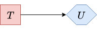
At this stage, the only remaining node is the decision node \(\textcolor{red}{T}\), which we can now eliminate by selecting the optimal action. The table below summarizes the optimal decision for \(\textcolor{red}{T}\), and Figure 14 shows the final influence diagram after its removal:
| $$\textcolor{red}{\delta^*(T)}$$ | $$\textcolor{blue}{U}$$ |
|---|---|
| no perform | 721 |

|
| Figure 14. Final influence diagram after removing decision node T. |
As we can see, this yields the same result as the decision tree in Part I: the company should not perform the test and should buy the oil field.
Influence Diagram Libraries
In practice, we do not need to manually perform each step of the arc-reversal or node-reduction algorithm to evaluate an influence diagram. Several open-source libraries automate this entire process and provide sophisticated inference algorithms that handle the computational complexity for us.
PyAgrum is currently the most widely supported open-source library for influence diagrams. Written in C++ with a Python interface, it implements the Shafer-Shenoy algorithm for LIMIDs (Shafer & Shenoy, 1990). PyAgrum builds a junction tree representation of the influence diagram and uses message passing, alternating between summation (for chance nodes) and maximization (for decision nodes), to efficiently evaluate the diagram.
Other notable libraries include:
-
GeNIe/SMILE: Implemented in C++, GeNIe is a useful, though somewhat dated, tool for working with Bayesian networks and influence diagrams. SMILE is the underlying engine. Both are free for academic use but are not open-source. -
PyCID: Written in Python, PyCID is a specialized open-source library designed for working with causal influence diagrams.
Conclusion
This post has shown how influence diagrams can be used to model and solve decision problems under uncertainty. By applying the arc-reversal and node-reduction algorithms to the oil-field LIMID, we obtained a maximum expected utility of 721 and confirmed that the optimal strategy is to skip the porosity test and buy the field. As expected, this matches the recommendation from the equivalent decision tree discussed in Part I.
Influence diagrams excel at capturing conditional independencies, which helps control the combinatorial explosion that often plagues decision trees. However, their main limitation is that they are best suited for symmetric problems. Highly asymmetric scenarios may require introducing artificial states or degenerate probabilities, which can increase both the size and computational complexity of the model.
In the next post, we’ll demonstrate how to build and evaluate LIMIDs using open-source tools like PyAgrum, perform sensitivity analysis and value-of-information calculations, and explore advanced features such as multiple utility nodes and decision planes. Finally, we’ll show how to integrate Gradio with PyAgrum to create interactive, web-based decision problem demos, making it easy to experiment with and communicate complex decision models.
References
- Shenoy, P. P. (2009). Decision trees and influence diagrams. Encyclopedia of life support systems, 280-298.
- Rodriguez, F. (2025, June 8). Introduction to decision theory: Part I.
- Wikipedia article on conditional independence.
- Wikipedia article on probability trees.
- Wikipedia article on Bayesian networks.
- Howard, R. A., & Matheson, J. E. (1984). Influence diagrams. The Principles and Applications of Decision Analysis (Vol. II), 719-762.
- Bielza, C., & Shenoy, P. P. (1999). A comparison of graphical techniques for asymmetric decision problems. European Journal of Operational Research, 119(1), 1-13.
- Lauritzen, S. L., & Nilsson, D. (2001). Representing and solving decision problems with limited information. Management Science, 47(9), 1235-1251.
- Shachter, R. D. (1986). Evaluating influence diagrams. Operations research, 34(6), 871-882.
- Wikipedia article on variable elimination.
- Jensen, F., Jensen, F. V., & Dittmer, S. (1994). From influence diagrams to junction trees. In Proceedings of the 10th Conference on Uncertainty in Artificial Intelligence (UAI) (pp. 367-373).
- Madsen, A. L., & Jensen, F. (1999). Lazy evaluation of symmetric Bayesian decision problems. In Proceedings of the Fifteenth Conference on Uncertainty in Artificial Intelligence (UAI) (pp. 382–390). Morgan Kaufmann.
- Shachter, R. D., & Kenley, C. R. (1989). Gaussian influence diagrams. Management Science, 35(5), 527–550.
- Jenzarli, A. (1995). Solving influence diagrams using Gibbs sampling. In Pre-proceedings of the Fifth International Workshop on Artificial Intelligence and Statistics (pp. 278-284). PMLR.
- Bielza, C., Müller, P., & Ríos-Insua, D. (1999). Decision analysis by augmented probability simulation. Management Science, 45(7), 995–1007.
- Cobb, B. R., & Shenoy, P. P. (2008). Decision making with hybrid influence diagrams using mixtures of truncated exponentials. European Journal of Operational Research, 186(1), 261-275.
- Winn, J., & Bishop, C. M. (2005). Variational message passing. Journal of Machine Learning Research, 6, 661–694.
- Shafer, G., & Shenoy, P. P. (1990). Probability Propagation. Annals of Mathematics and Artificial Intelligence, 2, 327-352.