Introduction to Decision Theory: Part I

Table of Contents

• The Challenge of Decision-Making
• The Anatomy of a Decision Problem
  • Structuring the Oil Field Decision Problem
  • Calculating Expected Monetary Value
  • Beyond Money: Utility and Risk Preferences
• Decision Analysis: A Dynamic, Iterative Process
• When New Information Becomes an Option
• Modelling the Problem with a Decision Tree
• Evaluating the Decision Tree
  • Perform the Test and the Result is "pass"
  • Perform the Test and the Result is "fail"
  • No Test Performed
  • Evaluating the Root Decision: Test vs. No Test
• Conclusion
• References

The Challenge of Decision-Making

Imagine you are the CEO of an oil company and you are offered the opportunity to purchase a new oil field. Like any diligent executive, you gather your team to examine satellite images, geological surveys, and consult the team’s experience with similar fields in the region.

This research helps form your initial assessment of the field’s potential. However, the reality is that until you actually start drilling, there’s no way to know for sure how much oil is down there. This leaves you with a classic dilemma:

• Play it safe and walk away.
• Make a calculated bet based on the evidence you’ve gathered.

Figure 1. Satellite imagery and heatmap of the oil field (source)

This tension between what you know, what you don’t know, and what you truly value is at the heart of every important decision. How do you weigh the potential upside against the risk of a bad draw? How much should your assessment count in the final call?

Decision Theory offers a framework to answer exactly these questions. It’s about systematically looking at the likelihood of different scenarios and weighing them against how much you value each potential result. By doing this, it guides you toward the action that’s most likely to give you the best overall outcome.

Let’s return to the oil field example. Suppose you’ve sized up the field and think it could fall into one of three quality levels:

• High, promising oil reserves.
• Medium, meaning a decent output but nothing groundbreaking.
• Low, where you’d barely break even or could even end up losing money.

The dilemma, then, becomes quite clear. If you decide to buy and the field turns out to be high-quality, you’ve struck gold. If you buy and it’s low-quality, you’ll lose your investment. But if you choose not to buy, you avoid any potential loss, though you might also miss out on a good opportunity.

The Anatomy of a Decision Problem

At its core, any decision problem can be broken down into a few fundamental components: the actions we can take, the uncertain conditions that might influence the outcome (often referred to as states of nature), the probabilities we assign to these conditions based on our best estimates, and the potential outcomes for each action under each condition.

So, let’s use the decision theory framework for our oil field case.

Structuring the Oil Field Decision Problem

First, what are the possible actions? The company faces a straightforward choice: either buy the oil field, investing capital now with the hope of future profits, or do not buy, which means avoiding the risk but also potentially missing out on gains.

Next, we consider the states of nature – the things we can’t control. In this case, it’s the true quality of the oil field. We’ve simplified this into three possibilities: the field could be high quality, medium quality, or low quality.

Then, we need to assign probabilities to these states. The company doesn’t know the field’s true quality for sure, but based on all the geological data and expert opinions, they’ve estimated the chances: a 35% chance of it being high quality, a 45% chance for medium quality, and a 20% chance for low quality.

Finally, let’s look at the outcomes, specifically the financial implications (in millions of dollars) for each scenario. These are summarized in the table below:

Action	Field Quality	Monetary Outcome
Buy	High	+$1250M
Buy	Medium	+$630M
Buy	Low	+$0M
Do not buy	Any	+$350M

Why is there a profit for not buying?

This could represent a baseline alternative, like investing the capital elsewhere for a guaranteed return of $350M.

Calculating Expected Monetary Value

So, how do we weigh these possibilities financially? A common approach is to calculate the Expected Monetary Value (EMV). For the ‘Buy’ option, the EMV considers each potential outcome, its likelihood, and its financial value. Here’s how it breaks down:

\[\begin{align*} \mathbb{E}[MV(\text{Buy})] &= (0.35 \cdot \$1250\text{M}) + (0.45 \cdot \$630\text{M}) + (0.20 \cdot \$0\text{M}) \\ &= \$437.5\text{M} + \$283.5\text{M} + \$0\text{M} \\ &= \$721\text{M} \end{align*}\]

This gives us an EMV of $721M if we decide to buy. Now, let’s look at the ‘Do not buy’ option. Its EMV is simpler:

\[\mathbb{E}[MV(\text{Do not buy})] = \$350\text{M}\]

Purely from an EMV perspective, buying the field seems to be the stronger choice, offering an expected $721M versus $350M.

Beyond Money: Utility and Risk Preferences

But EMV doesn’t always tell the whole story. What if not making a profit from this project could be disastrous for our company, or on the flip side, a big payout isn’t really necessary? EMV treats every dollar the same. However, real-world decisions often depend on how much risk we’re willing to take.

That’s where utility theory comes in. Instead of just looking at dollar amounts, we give each outcome a “utility score” to show how much it really matters to us. EMV assumes linear utility, which only holds if the decision maker is risk-neutral. Utility theory allows us to account for different risk preferences. Then we calculate an Expected Utility (EU) by weighing these scores by their probabilities (von Neumann & Morgenstern, 1944), just like we do with EMV.

So how do we figure out these utility scores? We start by anchoring the utility scale to simplify comparisons:

• Set best monetary outcome → \(U(\$1250\text{M}) = 1\)
• Set worst monetary outcome → \(U(\$0) = 0\)

Then, we need to find utility values for those outcomes in the middle ($350M, $630M). This depends on the decision maker’s risk preferences. One popular approach is the standard gamble. In this method, you ask the decision maker what probability of achieving the best outcome (i.e., $1250M) they would accept in a lottery compared to taking a guaranteed amount.

For instance, consider the $350M outcome:

“Would you rather take a sure $350M, or a gamble with a 70% chance of $1250M and 30% chance of $0M?”

If they say they’re indifferent, we assign: \(U(\$350\text{M}) = 0.7\).

Using the same logic for the $630M outcome:

“Would you rather take a sure $630M, or a gamble with a 90% chance of $1250M and 10% chance of $0M?”

If they express indifference here as well, then: \(U(\$630\text{M}) = 0.9\).

Action	Field Quality	Monetary Outcome	Utility Outcome
Buy	High	+$1250M	1
Buy	Medium	+$630M	0.9
Buy	Low	+$0M	0
Do not buy	Any	+$350M	0.7

Let’s compute the EU:

\[\begin{align*} &\mathbb{E}[U(\text{Buy})] = (0.35 \cdot 1.0) + (0.45 \cdot 0.9) + (0.20 \cdot 0.0) = 0.755 \\ \\ &\mathbb{E}[U(\text{Do not buy})] = 0.7 \end{align*}\]

EMV suggests to Buy ($721M > $350M). EU also suggests to Buy, but the margin is smaller (0.755 > 0.7). A more risk-averse person (e.g., someone with \(U(\$350\text{M})=0.8\)) would flip the decision.

Previous case is just a hypothetical example. For this article, we’ll keep things straightforward and assume the decision maker is risk neutral. Therefore, in our decision tree analysis below, we can use Expected Utility (EU) where utility values are directly proportional to monetary values, so a utility of 1000 corresponds to $1000M, etc. This makes EU and EMV equivalent for our analysis. In reality, though, considering non-linear utility can change which option looks best.

Another well-known example illustrating EMV’s limitations is the St. Petersburg Paradox. In this scenario, a casino offers a gamble where a fair coin is tossed until heads appears. If the first head appears on the nth toss, the prize is \(2^{n}\). Assuming the game continues indefinitely and the casino has unlimited resources, the EMV is infinite. This suggests one should pay any amount to play, yet most people wouldn’t pay more than $8 - $16. The reason is that the large payouts are so improbable that we mentally discount them, thus creating the paradox.

Decision Analysis: A Dynamic, Iterative Process

Decision-making isn’t a one-shot task. It’s a cycle of refinement. As new information emerges or priorities shift, we revisit and update our analysis. This structured approach ensures that our choices are not only well-founded but also adaptable.

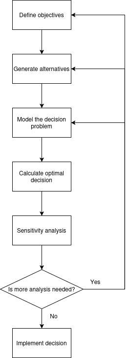
Figure 2. Flow diagram of the decision analysis process

The process begins with getting clear on what we’re trying to achieve. Instead of a vague goal like “maximize profits,” we break it down into specific, measurable objectives. For our oil company, this means not only aiming for the highest return but also minimizing downside risk, limiting upfront costs, and ensuring the project aligns with their strategic reserves.

With these objectives in mind, the next step is to brainstorm all feasible actions, not just the obvious ones. Beyond simply buying or not buying the field, perhaps there’s a third path, like delaying the decision to commission an extra study for more data.

Once the alternatives are on the table, we model the decision. This involves structuring the uncertainties (like the field’s quality), assigning probabilities (a 35% chance of high quality, etc.), and mapping outcomes to their values. This is where tools like decision trees and decision networks (i.e., influence diagrams) become useful for visualizing the entire problem.

With the model built, we can calculate the optimal path forward. As we saw, computing the EU helps us compare the options. Based on the EU, we know that buying is the stronger choice. But a good analysis doesn’t stop there. We need to ask, “what if?” This is the role of sensitivity analysis: testing how robust our decision is by tweaking the key inputs. What if the outcome for a “low quality” field isn’t breaking even, but a loss of $200M?

\[\mathbb{E}[U(\text{Buy})] = (0.35 \cdot 1250) + (0.45 \cdot 630) + (0.20 \cdot -200) = 681.5\]

The EU for buying is now 681.5, still the optimal choice, but the risk profile has clearly changed.

This stress-testing leads to the final step: implement or iterate. If the optimal choice proves robust and aligns with the company’s objectives, it’s time to move forward. But if the analysis reveals too much uncertainty or uncovers new risks, it’s a signal to revisit the earlier stages. Maybe the uncertainty is too high, and it’s worth gathering more data. Perhaps other variables, like environmental costs, need to be factored into the model. Or maybe new alternatives, like exploring a partnership to share the risk, have become more attractive.

When New Information Becomes an Option

Just as the company is about to move forward, a new opportunity arises: it can choose to perform a geological test before deciding whether to purchase the oil field. This test won’t reveal the true quality of the field, but it will measure the rock’s porosity, which measures how much empty space the rock contains that could hold oil. The test has two possible outcomes:

• Pass: Porosity is ≥ 15%, indicating a significant amount of pore (void) space in the rocks, which suggests a higher likelihood of finding oil.
• Fail: Porosity is < 15%, indicating less void space and therefore a lower potential for oil.

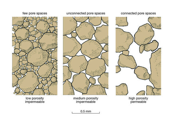
Figure 3. Reservoir quality illustrated through porosity and permeability characteristics (source)

In an ideal situation, the test would be extremely accurate. However, real-world tests are not perfect. The table below illustrates these measurement inaccuracies by presenting the conditional probability of each test result based on the quality of the oil field:

	high	medium	low
pass	0.95	0.7	0.15
fail	0.05	0.3	0.85

The test costs $30 million, and even after getting the results, the company still has to decide whether to buy the field. This means there are now two decisions to make: first, whether to conduct the test, and second, whether to purchase the field based on the test results. This kind of two-step decision-making, where each choice affects the next and involves probabilities, can’t be handled with simple payoff tables. Instead, we’ll need to use a decision tree or a decision network to figure it out.

Modelling the Problem with a Decision Tree

Decision trees, originating from the work of Raiffa & Schlaifer (1961), are a powerful tool for visualizing and analyzing decision-making problems. They map out the sequence of decisions and chance events, providing a clear picture of the possible outcomes and their associated probabilities. A decision tree consists of three types of nodes:

• Decision nodes. These are points where you need make a choice and take an action. In our case, the first decision here is whether to do the geological test. If the test is conducted, the next decision is whether to buy the oil field based on the test results.

• Chance nodes. These nodes represent states of nature or events that can affect the outcome. For our problem, the chance nodes include the possible results of the geological test and the actual quality of the oil field.

• Outcome nodes. These are the final nodes that show the result of a particular path through the tree.

To construct the tree, begin by identifying the root node, which represents the first event observed over time: either a decision or an uncertainty factor. From the root, add chance or decision nodes, outlining the different paths to follow, until you reach a terminal node, where the corresponding consequence will be indicated. The decision tree is then completed by including the utilities at the terminal nodes. At these nodes, a value is assigned to a final result, assuming this result has been achieved without considering probabilities.

Below is the decision tree for the oil drilling scenario. In this diagram, T represents the decision node for conducting the test, R indicates the test result, B denotes the decision to buy or not buy, and Q signifies the quality of the oil field.

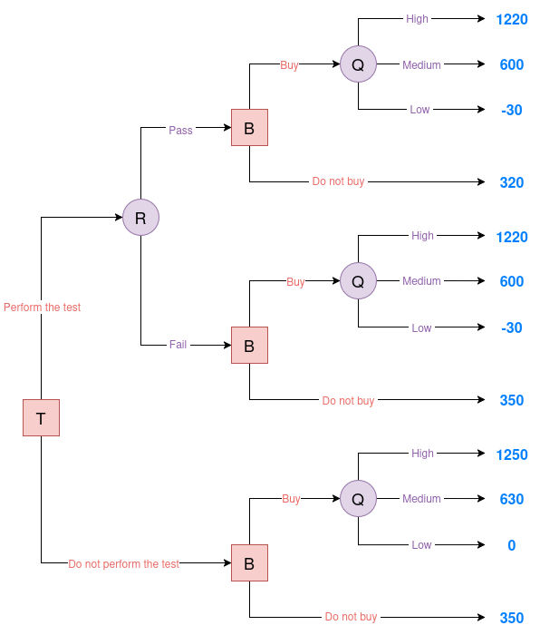
Figure 4. Oil decision tree

Evaluating the Decision Tree

To figure out the best course of action in a decision tree, we need to look at every possible decision path. This boils down to two key steps:

1. Estimating Probabilities. This involves using both marginal and conditional probabilities.
2. Calculating Expected Utilities. This requires evaluating the outcomes for each decision.

Same as before, the EU of a decision is computed by multiplying the utility of each outcome by its associated probability and summing these products across all possible outcomes under that decision. Since we’re assuming risk neutrality, utilities are proportional to monetary values. The decision with the highest EU at each decision node is the optimal choice.

Perform the Test and the Result is "pass"

From the test accuracy table, we know \(P(R \mid Q)\), which is the probability of each test result given the true field quality. But to evaluate the decision tree, we need the opposite: \(P(Q \mid R)\), the probability of each field quality given the observed test result. This is important because once we see the test result, we have to decide whether to buy based on the updated belief about the field quality. We’ll use Bayes’ Theorem to calculate these posterior probabilities of Q given that the test result is a “pass”.

First, we compute the marginal probability of obtaining a “pass” result:

\[\begin{align*} P(R = \text{pass}) &= P(R = \text{pass} | Q = \text{high}) \cdot P(Q = \text{high}) \\ &\quad + P(R = \text{pass} | Q = \text{medium}) \cdot P(Q = \text{medium}) \\ &\quad + P(R = \text{pass} | Q = \text{low}) \cdot P(Q = \text{low}) \\ &= 0.95 \cdot 0.35 + 0.7 \cdot 0.45 + 0.15 \cdot 0.20 = 0.3325 + 0.315 + 0.03 = 0.6775 \end{align*}\]

Then, we apply the theorem:

\[\begin{align*} P(Q = \text{high} \mid R = \text{pass}) &= \frac{0.95 \cdot 0.35}{0.6775} = 0.4908 \\ P(Q = \text{medium} \mid R = \text{pass}) &= \frac{0.7 \cdot 0.45}{0.6775} = 0.4649 \\ P(Q = \text{low} \mid R = \text{pass}) &= \frac{0.15 \cdot 0.20}{0.6775} = 0.0443 \end{align*}\]

We now compute the EU of buying the oil field after a “pass” result:

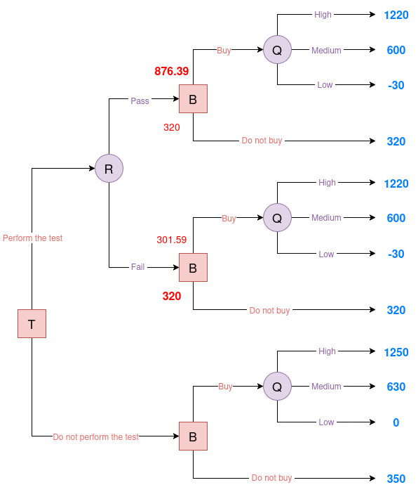
\[\mathbb{E}[U \mid R = \text{pass}, \text{Buy}] = 0.4908 \cdot 1220 + 0.4649 \cdot 600 + 0.0443 \cdot (-30) = 876.39\]

We compare the EU of buying versus not buying after a “pass” result:

• Buying: 876.39
• Not Buying: 320

Since 876.39 > 320, it is better to buy the oil field if the test result is pass.

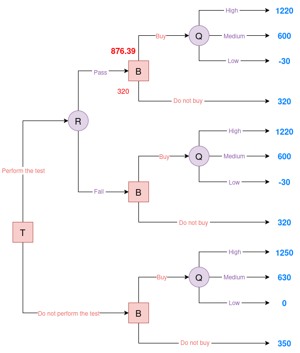
Figure 5. Evaluated Oil decision tree #1

Perform the test and the result is "fail"

As in the previous scenario, we first calculate the marginal probability of obtaining a “fail” result:

\[P(R = \text{fail}) = 1 - P(R = \text{pass}) = 1 - 0.6775 = 0.3225\]

Next, we apply Bayes’ Theorem to determine the posterior probabilities of Q given that the test result is “fail”:

\[\begin{align*} P(Q = \text{high} \mid R = \text{fail}) &= \frac{0.05 \cdot 0.35}{0.3225} = 0.0543 \\ P(Q = \text{medium} \mid R = \text{fail}) &= \frac{0.3 \cdot 0.45}{0.3225} = 0.4186 \\ P(Q = \text{low} \mid R = \text{fail}) &= \frac{0.85 \cdot 0.20}{0.3225} = 0.5271 \end{align*}\]

We then calculate the EU of purchasing the oil field after a “fail” result:

\[\mathbb{E}[U \mid R = \text{fail}, \text{Buy}] = 0.0543 \cdot 1220 + 0.4186 \cdot 600 + 0.5271 \cdot (-30) = 301.59\]

We compare the EU of buying versus not buying after a “fail” result:

• Buying: 301.59
• Not Buying: 320

Since 301.59 < 320, it is better to not buy the oil field if the test result is fail.

Figure 6. Evaluated Oil decision tree #2

No Test Performed

If the company decides not to conduct the porosity test, it must choose whether to purchase the oil field based solely on the prior probabilities of the field’s quality.

We calculate the EU of purchasing the field using the provided prior distribution for field quality:

\[\begin{aligned} \mathbb{E}[U \mid \text{No test}, \text{Buy}] &= 0.35 \cdot 1250 + 0.45 \cdot 630 + 0.20 \cdot 0 \\ &= 437.5 + 283.5 + 0 \\ &= 721 \\ \end{aligned}\]

We then compare the EU of buying versus not buying:

• Buying: 721
• Not Buying: 350

Since 721 > 350, it is better to buy the oil field if the company opts not to test.

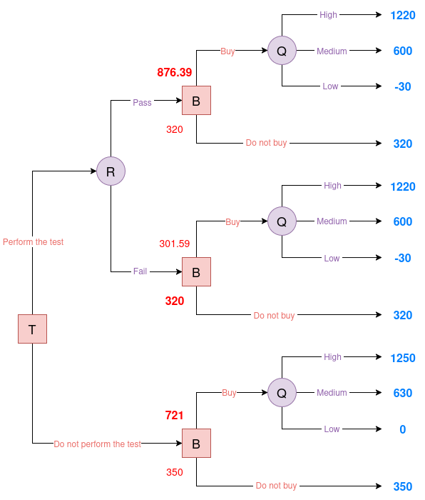
Figure 7. Evaluated Oil decision tree #3

Evaluating the Root Decision: Test vs. No Test

The final step is to determine whether the company should conduct the porosity test or proceed without testing. This hinges on comparing the EU of both options.

If the company performs the test, the overall EU is computed by weighting the outcomes of both possible test results:

\[\begin{aligned} \mathbb{E}[U \mid \text{Test}] &= P(R = \text{pass}) \cdot \mathbb{E}[U \mid R = \text{pass}] \\ &\quad + P(R = \text{fail}) \cdot \mathbb{E}[U \mid R = \text{fail}] \\ &= 0.6775 \cdot 876.39 + 0.3225 \cdot 320 \\ &= 696.95 \end{aligned}\]

Here, we assume the company buys the field if the test passes, and does not buy if it fails (i.e., the rational decision). Without conducting the test, the company’s best decision is to buy the field outright, resulting in an EU of 721.

We then compare the options:

• Test: 696.95
• No Test: 721

Since 721 > 696.95, the company should not perform the test and proceed directly to buy the oil field.

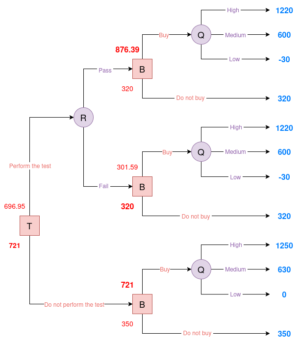
Figure 8. Evaluated Oil decision tree #4

Conclusion

In this post, we explored the foundations of decision theory through a practical investment scenario. We learned how to structure decision problems by identifying actions, uncertainties, probabilities, and outcomes. We looked at how to use EU to guide decision-making, and how risk preferences can shape the optimal choice. We also introduced decision trees as a valuable tool for analyzing sequential decisions under uncertainty, and showed how new information, such as a geological test result, can be incorporated into the analysis.

In the next post, we’ll discuss the limitations of decision trees and introduce decision networks, which offer a more compact and flexible way to represent complex decision problems with multiple variables and dependencies.

For more examples of decision analysis, check out:

• Ride-hailing subscription service: Should a ride-hailing company offer a retention deal to prevent customer churn?
• Logistics center automation: Should an e-commerce company upgrade its logistics center with robotics?

To read more about decision theory and its applications consider the following bibliography:

Book Cover	Reference	Key Focus
	Howard & Matheson (1983) Readings on Decision Analysis PDF link	Classic collection of papers on decision analysis methodology and applications
	Robert T. Clemens (1995) Making Hard Decisions	Practical guide to structuring decisions and handling uncertainty with real-world examples
	Ríos Insua et al. (2002) Fundamentos de los Sistemas de Ayuda a la Decisión	Comprehensive introduction to decision support systems with emphasis on theoretical foundations
	Koller & Friedman (2009) Probabilistic Graphical Models (Ch. 22, 23) PDF Link	Advanced coverage of decision networks and their integration with probabilistic reasoning
	Russell & Norvig (2010) AI: A Modern Approach (Ch. 16) PDF Link	Introduction to decision theory & decision networks

References

1. Wikipedia page on decision theory.
   
   
2. Stanford’s Encyclopedia page on utility theory.
   
   
3. von Neumann J., Morgenstern, O. (1944). Theory of Games and Economic Behavior. Princeton University Press.
   
   
4. Ontosight article on standard gamble.
   
   
5. Wikipedia article on St. Petersburg Paradox.
   
   
6. Wikipedia article on decision trees.
   
   
7. Wikipedia article on decision networks.
   
   
8. Wikipedia article on sensitivity analysis.
   
   
9. Raiffa, H., Schlaifer, R. (1961). Applied statistical decision theory. John Wiley & Sons.