• Can language models think "probabilistically"?
• Bayesian networks
• Probabilistic inference on Bayesian networks
• Variable Elimination algorithm
  • Operations on factors
  • The algorithm
  • Example
    • Step 1: Restrict factors based on evidence
    • Step 2: Eliminate V2
    • Step 3: Eliminate V0
    • Step 4: Normalize
• How LLMs do it
  • Experimental setup
  • Raw reasoning results
  • Code generation results
• Conclusion
• References

Can language models think "probabilistically"?

This question has been on my mind for a while. It motivated me to revisit probabilistic graphical models, write my blog series on Decision Theory, and explore how large language models (LLMs) solved a few hand-crafted decision problems.

Early experiments were promising: models like O3 and Gemini-2.5-Pro reached correct solutions on small decision problems. But I observed they were solving them using decision trees, which have theoretical limitations. I wondered: were LLMs using decision trees because it was “easier”, or because they didn’t know how to apply influence diagrams?

To answer that, I started running more extensive experiments. But midway through, I realized I was getting ahead of myself. If I wanted to evaluate LLMs on influence diagrams, I should probably start with Bayesian networks, since influence diagrams are essentially Bayesian networks augmented with decisions and utilities. If LLMs struggle with probabilistic inference on Bayesian networks, expecting them to solve full decision problems could be premature.

So that’s what this post explores: how do current frontier LLMs handle probabilistic inference on a Bayesian network? I’ll walk through the Variable Elimination algorithm since it is one of the easiest to understand and implement, solve an example by hand with it, and then compare how seven reasoning LLMs approach the same query, analyzing not just whether they get the right answer, but how they reason through the problem.

Bayesian networks

A Bayesian network (BN) is a directed acyclic graph (DAG) in which nodes represent random variables. Arcs encode conditional dependencies between variables in a way that allows us to factorize the joint probability distribution into a product of conditional probability distributions (CPDs),

where \(\mathbf{Pa}_{\textcolor{purple}{V_i}}\) denotes the parents of variable \(\textcolor{purple}{V_i}\) in the DAG. This property is often called the chain rule for Bayesian networks.

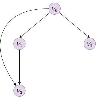
As an example, consider a Bayesian network with 4 binary variables (\(\textcolor{purple}{V_0}, \textcolor{purple}{V_1}, \textcolor{purple}{V_2}, \textcolor{purple}{V_3}\)). The structure is a simple diamond-like shape where \(\textcolor{purple}{V_0}\) is the root, \(\textcolor{purple}{V_1}\) and \(\textcolor{purple}{V_2}\) depend on \(\textcolor{purple}{V_0}\), and \(\textcolor{purple}{V_3}\) depends on both \(\textcolor{purple}{V_0}\) and \(\textcolor{purple}{V_1}\).

Figure 1. Bayesian network example with 4 variables

Probabilistic inference on Bayesian networks

Once we have a BN, we can use it to reason by performing probabilistic inference. This task involves computing the probability of query variables \(\mathbf{\textcolor{purple}{Q}}\) given some observed evidence \(\mathbf{\textcolor{purple}{E}} = \mathbf{\textcolor{purple}{e}}\).

Theoretically, this is straightforward. The Bayesian network defines the full joint distribution, so we could sum over all unobserved “nuisance” variables \(\mathbf{\textcolor{purple}{Z}}\):

However, this naive approach is computationally infeasible. For a network with \(n\) binary variables, storing the full joint distribution would require a table with \(2^n\) entries.

Instead of storing that massive table, we can use the BN factorization (Equation 1) to compute only the specific joint probabilities we need on-the-fly. By substituting the factorization into Equation (2), we get:

While this saves us from storing the full table, we still face the problem of summing over it. We still need to enumerate all combinations of hidden variables \(\mathbf{\textcolor{purple}{z}}\). For 30 binary variables, that’s over a billion terms to sum. This approach, often called inference by enumeration or simply applying the chain rule naively, is conceptually simple but does not scale.

Efficient inference algorithms avoid this exponential blowup by exploiting the factorized representation more cleverly. Rather than enumerating all combinations, they manipulate the individual CPDs (which are much smaller) and perform marginalization locally, pushing sums inside products where conditional independence allows. Well-known examples include Variable Elimination, Junction Tree algorithm, and Belief Propagation (Koller & Friedman, 2009). We’ll focus on Variable Elimination since it’s the easiest to explain and commonly used when teaching BN inference.

Variable Elimination algorithm

As the name suggests, the Variable Elimination (VE) algorithm works by eliminating the variables of the network until it yields the answer to a specific query. This algorithm is typically defined in terms of factors.

A factor \(\phi(\mathbf{\textcolor{purple}{X}})\) is a function that maps a set of variables \(\mathbf{\textcolor{purple}{X}}\) to a real positive value. CPDs are an example of factors. In fact, the initial set of factors corresponds exactly to the CPDs of the network.

During inference, new factors are created by multiplying and marginalizing existing ones. These intermediate factors are generally unnormalized, meaning their values do not sum to one. This is not a problem, since normalization is only required for the final result. Working with unnormalized factors simplifies computation and allows inference algorithms to focus on local operations.

Operations on factors

VE relies on three operations:

1. Factor Product: Combine two factors \(\phi_1(\textcolor{purple}{V_1})\) and \(\phi_2(\textcolor{purple}{V_2})\) into a new factor \(\phi_{new}\) over \(\textcolor{purple}{V_1} \cup \textcolor{purple}{V_2}\) by multiplying their values for every consistent assignment:

1. Marginalization: Eliminate a variable \(\textcolor{purple}{Z}\) from factor \(\phi(\textcolor{purple}{V}, \textcolor{purple}{Z})\) by summing over all its values to produce a new factor \(\phi_{new}\):

   \[\phi_{new}(\textcolor{purple}{V}) = \sum_{\textcolor{purple}{z}} \phi(\textcolor{purple}{V}, \textcolor{purple}{Z} =\textcolor{purple}{z})\]

2. Evidence restriction: If variable \(\textcolor{purple}{E}\) is observed to be \(\textcolor{purple}{e}\), restrict any factor containing \(\textcolor{purple}{E}\) to that value, essentially selecting the slice of the table consistent with the observation.

The algorithm

Given a Bayesian network, query variables \(\mathbf{\textcolor{purple}{Q}}\), and evidence \(\mathbf{\textcolor{purple}{E}} = \mathbf{\textcolor{purple}{e}}\):

1. Initialize: Treat each CPD as a factor. Restrict all factors to be consistent with the evidence \(\mathbf{\textcolor{purple}{E}} = \mathbf{\textcolor{purple}{e}}\).

2. Choose elimination order: Pick an ordering for the hidden variables \(\mathbf{\textcolor{purple}{Z}}\) (neither query nor evidence). The choice of ordering affects efficiency because bad orders create large intermediate factors.

1. Eliminate variables: For each variable \(\textcolor{purple}{Z_i}\) in order:
   • Collect all factors containing \(\textcolor{purple}{Z_i}\)
   • Multiply them into a single factor \(\phi_{new}'\)
   • Sum out \(\textcolor{purple}{Z_i}\) to get a new factor \(\phi_{new}''\)
   • Replace the collected factors with \(\phi_{new}''\)
2. Normalize: Multiply remaining factors (now only over \(\mathbf{\textcolor{purple}{Q}}\)) and normalize to obtain \(P(\mathbf{\textcolor{purple}{Q}} = \mathbf{\textcolor{purple}{q}} \mid \mathbf{\textcolor{purple}{E}} = \mathbf{\textcolor{purple}{e}})\).

Example

As an example we are going to use the BN we defined in Figure 1 and compute the probability of \(\textcolor{purple}{V_3}\) being \(\textcolor{purple}{s_1}\) given that \(\textcolor{purple}{V_1}\) is observed to be \(\textcolor{purple}{s_0}\):

The evidence is \(\mathbf{\textcolor{purple}{E}} = \{\textcolor{purple}{V_1} = \textcolor{purple}{s_0}\}\). The query variable is \(\mathbf{\textcolor{purple}{Q}} = \{\textcolor{purple}{V_3}\}\). The hidden variables to eliminate are \(\mathbf{\textcolor{purple}{Z}} = \{\textcolor{purple}{V_0}, \textcolor{purple}{V_2}\}\).

We start with the initial factors (the CPDs):

For the elimination order, we have randomly selected to start with \(\textcolor{purple}{V_2}\) and then \(\textcolor{purple}{V_0}\).

Step 1: Restrict factors based on evidence

Since we observe \(\textcolor{purple}{V_1} = \textcolor{purple}{s_0}\), we restrict any factor containing \(\textcolor{purple}{V_1}\) to this value.

For \(\phi_1(\textcolor{purple}{V_1}, \textcolor{purple}{V_0})\), we fix \(\textcolor{purple}{V_1} = \textcolor{purple}{s_0}\). Since \(\textcolor{purple}{V_1}\) is now a constant, the resulting factor depends only on \(\textcolor{purple}{V_0}\). We call this new factor \(\phi_1'(\textcolor{purple}{V_0})\):

For \(\phi_3(\textcolor{purple}{V_3}, \textcolor{purple}{V_0}, \textcolor{purple}{V_1})\), we similarly select the entries consistent with \(\textcolor{purple}{V_1} = \textcolor{purple}{s_0}\). The new factor depends only on \(\textcolor{purple}{V_3}\) and \(\textcolor{purple}{V_0}\):

Step 2: Eliminate V2

The only factor containing \(\textcolor{purple}{V_2}\) is \(\phi_2(\textcolor{purple}{V_2}, \textcolor{purple}{V_0})\). Summing over \(\textcolor{purple}{V_2}\):

Since \(\textcolor{purple}{V_2}\) is a leaf node and not part of the query or evidence, it sums to 1 and effectively disappears (it is a “barren node”).

Step 3: Eliminate V0

We collect all factors containing \(\textcolor{purple}{V_0}\): \(\phi_0(\textcolor{purple}{V_0})\), \(\phi_1'(\textcolor{purple}{V_0})\), and \(\phi_3'(\textcolor{purple}{V_3}, \textcolor{purple}{V_0})\). We multiply them to form \(\phi_{prod}(\textcolor{purple}{V_3}, \textcolor{purple}{V_0})\):

For \(\textcolor{purple}{V_0} = \textcolor{purple}{s_{0}}\):

For \(\textcolor{purple}{V_0} = \textcolor{purple}{s_{1}}\):

Then we sum out \(\textcolor{purple}{V_0}\) to get \(\phi_5(\textcolor{purple}{V_3})\):

Step 4: Normalize

Finally, we normalize \(\phi_5(\textcolor{purple}{V_3})\) to get the probability distribution.

How LLMs do it

Now that we have solved the problem manually, let’s see how LLMs approach the task. To evaluate this comprehensively, I have prepared two complementary experiments:

1. Raw reasoning: Provide the network definition with CPDs in the prompt and ask for the answer without any tools. This tests whether LLMs can apply inference algorithms (Variable Elimination, Junction Tree, brute force, etc.) and perform arithmetic operations correctly. It’s essentially a test of what I did above but without a calculator (which I used).

2. Code generation: Provide the network definition with CPDs in the prompt and ask LLMs to write Python code to solve the problem. Given that current reasoning models have demonstrated excellent coding capabilities, this tests their ability to translate the problem into code and solve it. This is a “one-shot” test. I want to see what kind of code they would generate and how many output tokens are required compared to the raw reasoning approach.

Experimental setup

I have selected seven state-of-the-art language models, including both open-source and closed-source reasoning models. The experiments have been conducted using OpenRouter.

Models evaluated:

The complete experimental code is available in the code/llms-probabilistic-reasoning/ directory. Running the experiments requires only a few OpenRouter credits, and I’ve shared all results as JSON files for analysis under the results sub-directory.

Each experiment uses a different prompt, both defined in the prompts.yaml file. The raw reasoning template is prompt_base and the code generation template is prompt_base_code.

Raw reasoning results

All models successfully computed the correct probability. However, to be honest, that was not especially surprising. Reasoning models have shown great performance on math benchmarks in recent years, and the example query is not especially complicated given the size of the network. What is particularly interesting to me is how each model approached the task.

To analyze their approaches, I reviewed the traces and used Gemini-3-Pro to compare them against the VE algorithm I manually applied above. Note that for Gemini-3 and GPT-5.2 we only have access to reasoning “summaries” rather than the full thinking trace, so the analysis of these models is not as accurate.

As a summary, none of the models used the VE algorithm. Instead, all models except GPT-5.2 essentially wrote out the formula for the full joint distribution and then summed it up.

DeepSeek-R1, Kimi-K2, Sonnet-4.5, and Gemini-3 wrote the full joint distribution using the chain rule and brute-forced the summation. This forced them to re-calculate the same sub-problems multiple times (e.g., computing the probability of the parents for both the numerator and denominator separately). This redundancy is a major driver of token bloat.

GLM-4.7 and Qwen-3 also summed over the full joint distribution, but they realized that the numerator and denominator shared common terms, like \(P(\textcolor{purple}{V_0})P(\textcolor{purple}{V_1} \mid \textcolor{purple}{V_0})\), so they explicitly calculated these “blocks” once and reused them, naming them for example term1 and term2. However, while they avoid re-multiplying the same numbers, they are still committed to a formula that grows exponentially with the network size.

Finally, GPT-5.2 is the only one that truly changed the structure of the problem. It seems to me that it has applied Cutset conditioning. The idea is to find the minimal set of nodes whose instantiation will make the remainder of the network “singly connected” (i.e., a polytree). Once we have a tree, inference is easy and efficient. In this case, GPT-5.2 correctly identified that \(\textcolor{purple}{V_0}\) acts as a cutset (of size 1). Instantiating \(V_0\) breaks the connection between the “left” path (\(\textcolor{purple}{V_1}\)) and “right” path (\(\textcolor{purple}{V_2}\)). After it solved a small problem (finding \(\textcolor{purple}{V_0}\)’s posterior), it then used that answer to solve the next small problem (finding \(\textcolor{purple}{V_3}\)). To be honest, I was impressed by this. This is what I was hoping to see: LLMs using their reasoning capabilities to find “heuristics” to simplify the inference problem.

Code generation results

All models achieved the correct numerical answer. However, despite the prompt explicitly mentioning the possibility to write code for pgmpy and pyAgrum, none of the models used these established BN libraries. Instead, they all followed the same pattern: they derived the chain rule formula and implemented it using vanilla Python.

Looking at the traces, most models actually computed the answer (or at least verified their approach) manually before writing any code. Kimi-K2 and GPT-5.2 were the most extreme examples. They performed the full calculation by hand, including manual long division to many decimal places. Their code then used high-precision arithmetic (fractions.Fraction for Kimi-K2, decimal.Decimal with 50-digit precision for GPT-5.2), essentially double-checking their mental work rather than delegating the computation. On the other side of the spectrum, DeepSeek-R1 also computed the numerator and denominator but not the final result, which is why it was far more token efficient.

From my personal tests, I know these models are aware of pgmpy and pyAgrum and can write code using them. However, they seem to prefer direct calculations. Perhaps they find them more explainable or maybe they didn’t see it necessary for a small network like this one.

As an example, here is the resulting Python code from Sonnet-4.5 (all of them are quite similar):

# Calculate P(V3=s1 | V1=s0)

# P(V0)
P_V0_s0 = 0.5072
P_V0_s1 = 0.4928

# P(V1 | V0)
P_V1_s0_given_V0_s0 = 0.3110
P_V1_s0_given_V0_s1 = 0.0704

# P(V3 | V0, V1)
P_V3_s1_given_V0_s0_V1_s0 = 0.9393
P_V3_s1_given_V0_s1_V1_s0 = 0.1110

# Calculate P(V3=s1, V1=s0) using law of total probability
P_V3_s1_V1_s0 = (P_V3_s1_given_V0_s0_V1_s0 * P_V1_s0_given_V0_s0 * P_V0_s0 + 
                 P_V3_s1_given_V0_s1_V1_s0 * P_V1_s0_given_V0_s1 * P_V0_s1)

# Calculate P(V1=s0)
P_V1_s0 = P_V1_s0_given_V0_s0 * P_V0_s0 + P_V1_s0_given_V0_s1 * P_V0_s1

# Calculate P(V3=s1 | V1=s0)
result = P_V3_s1_V1_s0 / P_V1_s0

print(result)

For comparison’s sake, here’s how the problem could be solved using pgmpy. This is what I have considered ground truth for this experiment:

from pgmpy.inference import VariableElimination
from pgmpy.models import DiscreteBayesianNetwork
from pgmpy.factors.discrete import TabularCPD

# Create the Bayesian network structure
bn = DiscreteBayesianNetwork([('V0', 'V1'), ('V0', 'V2'), ('V0', 'V3'), ('V1', 'V3')])

# Define CPDs based on the provided tables

# CPD for V0 (root node)
cpd_v0 = TabularCPD(
    variable='V0',
    variable_card=2,
    values=[[0.5072], [0.4928]],
    state_names={'V0': ['s0', 's1']}
)

# CPD for V1 (depends on V0)
cpd_v1 = TabularCPD(
    variable='V1',
    variable_card=2,
    values=[[0.3110, 0.0704],
            [0.6890, 0.9296]],
    evidence=['V0'],
    evidence_card=[2],
    state_names={'V1': ['s0', 's1'], 'V0': ['s0', 's1']}
)

# CPD for V2 (depends on V0)
cpd_v2 = TabularCPD(
    variable='V2',
    variable_card=2,
    values=[[0.8950, 0.0562],
            [0.1050, 0.9438]],
    evidence=['V0'],
    evidence_card=[2],
    state_names={'V2': ['s0', 's1'], 'V0': ['s0', 's1']}
)

# CPD for V3 (depends on V0 and V1)
cpd_v3 = TabularCPD(
    variable='V3',
    variable_card=2,
    values=[[0.0607, 0.8173, 0.8890, 0.2251],
            [0.9393, 0.1827, 0.1110, 0.7749]],
    evidence=['V0', 'V1'],
    evidence_card=[2, 2],
    state_names={'V3': ['s0', 's1'], 'V0': ['s0', 's1'], 'V1': ['s0', 's1']}
)

# Add CPDs to the bn
bn.add_cpds(cpd_v0, cpd_v1, cpd_v2, cpd_v3)

# Validate the bn
assert bn.check_model()

# Create inference object
inference = VariableElimination(bn)

# Compute P(V3=s1 | V1=s0)
query_result = inference.query(variables=['V3'], evidence={'V1': 's0'})
prob_v3_s1_given_v1_s0 = query_result.values[1]  # Index 1 corresponds to V3=s1

print(prob_v3_s1_given_v1_s0)

Writing code using the chain rule for a small network is not “bad” per se, but it may suggest that these models are not accustomed to using BN libraries. This could be an issue for more complex queries, where translating the problem manually becomes error-prone or even infeasible.

A more significant observation is that every model chose to solve the inference problem manually before writing a single line of code. This “double-work”, combined with the verbose chain-rule derivation, leads to token bloat. Since reasoning LLMs have limited context windows and generation speeds (often 50-100 tokens/s), reducing this manual verification would make the process far more efficient. For instance, some responses took over 10-15 minutes to complete purely due to this verbosity.

Now, I don’t want to be all “doom and gloom”. First, this is based on a single example, and more experiments are needed. Second, I think these results are very interesting and hint at notable opportunities for optimization (e.g., training LLMs to use these BN libraries more often), especially as we move from pure LLMs to agents with iterative reasoning processes and tools.

Conclusion

The key takeaway from this exploration is that LLMs can solve probabilistic inference problems, but they currently do so inefficiently. Rather than applying BN algorithms like VE, they seem to prefer to write the chain rule formula and brute-force the arithmetic. This works for small networks but does not scale.

Limitations. This was a small-scale exploration with a single query on a 4-node network. A systematic evaluation would require varying network sizes, query complexities, and prompting strategies. I also did not test function calling, which would enable a more agentic approach.

Related work. While I have not found many papers on the topic, two recent papers are relevant: Paruchuri et al. (2024) evaluated LLMs on probabilistic reasoning over univariate distributions. Nafar et al. (2025) is closer to my experiments, testing how LLMs translate text-based probabilistic queries into symbolic representations.

Looking ahead. More experiments are needed: testing different network structures, varying sizes, and exploring alternative prompting strategies. I would also like to evaluate tool-augmented approaches via function calling, which could reveal whether LLMs perform better when they can delegate computation rather than doing it “in their heads.”

More broadly, understanding how LLMs reason “under the hood” about structured mathematical problems like probabilistic inference is valuable in itself. It helps us identify where current architectures struggle and what kinds of reasoning they handle well. This connects to a fascinating discussion on the Machine Learning Street Talk channel that I watched the other day, where researchers explore why LLMs still fail at arithmetic that a second-grader could do, and whether mathematical frameworks like Category Theory could help us understand these limitations more rigorously. It is a bit dense, but I recommend watching it if you are interested in the topic.

References

1. Rodriguez, F. (2025, July 4). Introduction to decision theory: Part II.
   
   
2. Rodriguez, F. (2025, August 7). Introduction to decision theory: Part III.
   
   
3. Koller, D., & Friedman, N. (2009). Probabilistic Graphical Models: Principles and Techniques. MIT Press.
   
   
4. Cutset conditioning lecture notes from Imperial College London. PDF link.
   
   
5. Nafar, A., Venable, K. B., & Kordjamshidi, P. (2025). Reasoning over uncertain text by generative large language models. In Proceedings of the AAAI Conference on Artificial Intelligence (Vol. 39, No. 23, pp. 24911-24920).
   
   
6. Paruchuri, A., Garrison, J., Liao, S., et al. (2024). What are the odds? Language models are capable of probabilistic reasoning. In Proceedings of the 2024 Conference on Empirical Methods in Natural Language Processing (pp. 11712-11733).
   
   
7. pgmpy documentation: https://pgmpy.org/.

Anyway, in one of those sporadic moments (this Sunday morning, to be precise), I glanced at my own profile text and remembered a conversation I had with my girlfriend this week about what a CV profile should say. Out of curiosity (and habit), I couldn’t help thinking to myself: What would Karpathy do? What does Karpathy have in his Linkedin profile? So I typed “karpathy” in the search bar, but when I was about to click on his profile, I misclicked and searched the term instead, allowing Linkedin to show me the “closest” thing to “karpathy” on the platform.

Figure 1. What would Andrej Karpathy do?

To my honest surprise, the top result was not Andrej Karpathy’s profile (could it be because he doesn’t post on Linkedin?). Instead, it was a post from an AI influencer.

Following my curiosity, I opened his profile to see what made his post the closest thing to “karpathy” (I am always on an almost “obsessive” mission to find interesting people and papers in the AI space, so I had to check). Inside, I saw he had 1.5M followers which could explain the recommendation. That shifted my curiosity: I decided to investigate how a “top voice” in the AI space actually writes, especially now that I’m dedicating some time to writing myself.

Reading one of the posts, I couldn’t help but notice common patterns of AI writing:

• Using a question in the middle of the post to catch the reader’s attention
• Phrases like “The more powerful the blablabla, the more human the blublublu…”
• Emojis or uncommon UTF-8 characters

Figure 2. Closest post to "karpathy" according to Linkedin search

Now, while my first intuition was that AI had played a role here, I am not a native English speaker, nor am I an expert on the topic. In fact, there is an interesting conversation to be had about how LLMs are influencing the way we speak. For instance, I have noticed myself using terms like “delve” and “showcase” more frequently, terms usually associated with AI writing, even when I am not using an LLM (Wikipedia has an interesting article about signs of AI writing, if you’re curious).

That said, I don’t believe that using LLMs means everything written or created will be slop. Nor do I think LLMs are “incapable” of creating creative or high-quality content, though there is certainly a discussion to be had about it (Jessica Hullman has an interesting blog post on the matter).

But I am slightly digressing. Coming back to that Linkedin post, I think it reignited an internal questioning I have been wrestling with all year about creativity and “craft”, especially with current AI advancements. Why do I build software? Why do I paint miniatures? Why spend a Sunday writing this post when an LLM could generate a “passable” version in seconds? To me, it boils down to two things: understanding why I create in the first place, and figuring out how to preserve myself in the resulting creation.

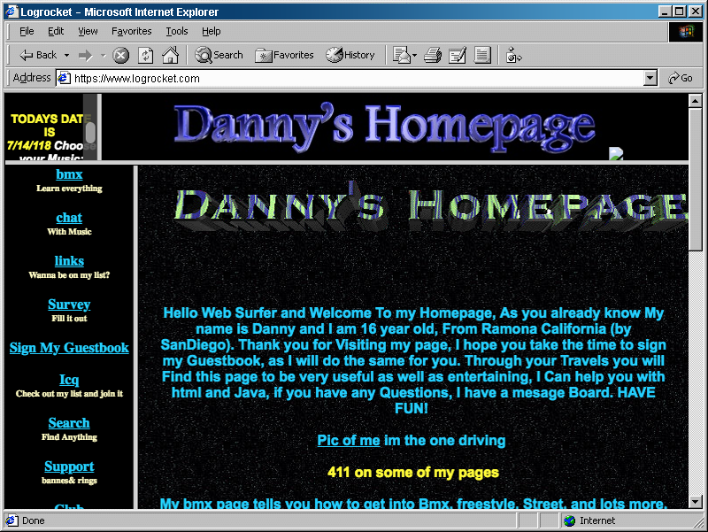
Thinking about all of this made me remember something I built long before LLMs existed: my first webpage, made back in 2006 for the game Metroid Prime Hunters. A page built using Microsoft FrontPage that, if I recall correctly, was hosted by Telecable, my home’s internet provider when I was a kid. I still remember the feeling of joy when I got it to work and shared the webpage with my friends.

Back then, there were no LLMs, not even StackOverflow, so I remember reading through the book and dedicating part of my weekends to learning and building through trial and error. I remember searching for the “coolest” images and GIFs on the internet, like the legendary “Dancing Banana GIF”: .

Unfortunately, I didn’t save a copy of that webpage, but it was something similar to the following:

Figure 3. A similar kind of webpage to the one I created when I was young (left) and my father's copy of Microsoft FrontPage (2002), which I used to build it (right)

When I think about that webpage, the miniatures I paint, these blog posts, and even the software I write every day in my job, I realize that what motivates me is creating something that is not only cool, but that also endures (even if just a little) and keeps a part of me in it.

This desire for endurance might be why “AI-accelerated” content often bothers me. It gives off a “fast-food” feeling, where things are created with no intention of lasting. It might be code without proper architecture or content designed solely to optimize for engagement algorithms and rise higher in the feed. On this topic, I remembered a conversation between Jeremy Howard and Chris Lattner about building software that lasts in an age when “everyone is vibe-coding their way through problems”.

So yeah, I think my main reflection here is about how we can use AI as a tool without losing ourselves in the process. I have been using LLMs to review my text and code since Chat-GPT was released in 2022. It is a learning process, but if used correctly, I don’t think using AI makes the result less “mine”.

As an example, here’s a cover letter I sent to Perplexity back in 2023 (I don’t think they’ll mind sharing it, they never replied). At the time, using an LLM for this felt almost novel to me, an experiment at integrating this new technology into my daily life. Reading the letter now, I still recognize my voice in it, even if I used an LLM to co-write it.

Figure 4. Cover letter I wrote back in 2023 for an application to Perplexity AI

One last analogy (I promise). I think current LLMs present a problem similar to the Ring of Gyges (here is a nice video from TED Ed that I found the other day, which motivated the example). In Plato’s story, the ring grants its wearer invisibility, and with it, the temptation to act without consequences. I think something similar happens with LLMs: we get a nice powerup and assume no one will notice. But even if that were true (and it’s doubtful, since remaining unnoticed is hard when everyone knows you have “the ring”), the real danger isn’t getting caught. It’s the risk of corruption, of slowly losing part of ourselves in the process.

For all these reasons, I like to remind myself why I do what I do. And I keep coming back to the same answer: I want to create something interesting that lasts. I write posts not just to share, but to organize and reflect on my ideas. I paint miniatures because the result is cool, tangible, and lasting. As for studying and working in AI, it helps me understand myself better as a human being and, honestly, I still dream of creating intelligent beings. With that clarity, LLMs, and AI in general, become useful tools that help me develop my “craft”, serving my goals rather than eroding my sense of self.

So, what about the original question? What does Karpathy have in his Linkedin profile? Well, his profile simply has the URL of his personal webpage, which probably makes sense for someone of his caliber. I am not sure if I should do the same, to be honest. Nevertheless, that small missclick finally pushed me to organize these thoughts. It also reminded me of what I wrote in that old cover letter. Now, hopefully, I can make a cool and lasting contribution, if not to AI itself, then at least with it.

• Closing the Loop
• Building the Oil-Field LIMID in PyAgrum
  • Setting Up the Network Structure
  • Filling in the Numbers
  • Solving the Network
• Testing Robustness with Sensitivity Analysis
  • Single Parameter Sensitivity Analysis
    • Example 1: Prior Probability of High-Quality Fields
    • Example 2: Test Precision for Medium-Quality Fields
  • Tornado Diagrams: Visualizing Parameter Impact
    • Example 1: Direct Utility Value Sensitivity
    • Example 2: Test Cost Sensitivity
  • Interactive Gradio Interface
    • Implementation Overview
    • Demo
• Conclusion
• References

Closing the Loop

In Part I, we explored the oil company’s dilemma: should we buy the field or walk away? We used a decision tree to analyze the problem step by step, weighing probabilities and payoffs to determine the optimal choice. In Part II, we examined the limitations of decision trees and introduced influence diagrams as a more scalable alternative. We solved the same problem manually using influence diagrams, confirming that they yield the same result as decision trees.

But let’s be honest, constantly redrawing diagrams and recalculating expected utilities every time geological estimates change or market conditions shift is not realistic. Real-world decision problems need tools that adapt quickly. That’s what we’ll build in this final part, focusing on two crucial questions:

1. How do we actually implement these models in code? We’ll see how to recreate our oil field analysis using PyAgrum, transforming those tedious manual calculations into just a few lines of Python.

2. How much should we trust the model’s recommendation? Using sensitivity analysis, we’ll discover whether our “buy the field” decision is robust to parameter changes. We’ll build different types of visualizations and create an interactive Gradio interface where we can adjust any parameter and immediately see the impact.

Building the Oil-Field LIMID in PyAgrum

PyAgrum is a Python wrapper around the C++ aGrUM library for building and solving probabilistic graphical models such as Bayesian networks, LIMIDs, causal networks, and more. With a few lines of Python code we can define the influence diagram’s structure, add the probabilities and utilities, execute, and get the optimal policy.

Let’s now code the decision problem.

Setting Up the LIMID Structure

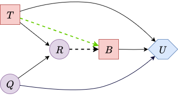
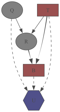
We start by importing pyagrum and creating an empty influence diagram. Then we add our four variables: oil field quality (\(\textcolor{purple}{Q}\)), test results (\(\textcolor{purple}{R}\)), the test decision (\(\textcolor{red}{T}\)), the buy decision (\(\textcolor{red}{B}\)), and a utility node (\(\textcolor{blue}{U}\)).

import pyagrum as grum
from pyagrum import InfluenceDiagram

# Create the influence diagram
influence_diagram = InfluenceDiagram()

# Initialize with 0 states, then manually add the labels we need
Q = influence_diagram.addChanceNode(
    grum.LabelizedVariable("Q", "Q", 0).addLabel('high').addLabel('medium').addLabel('low'))
R = influence_diagram.addChanceNode(
    grum.LabelizedVariable("R", "R", 0).addLabel('pass').addLabel('fail').addLabel('no_results'))
T = influence_diagram.addDecisionNode(
    grum.LabelizedVariable("T", "T", 0).addLabel('do').addLabel('not_do'))
B = influence_diagram.addDecisionNode(
    grum.LabelizedVariable("B", "B", 0).addLabel('buy').addLabel('not_buy'))
U = influence_diagram.addUtilityNode("U")  # Utility node takes just a name

Next, we connect the nodes with arcs to capture the dependencies from our diagram. Notice the memory arc from \(\textcolor{red}{T}\) to \(\textcolor{red}{B}\) that transforms the diagram into a LIMID.

# Add arcs to define dependencies
influence_diagram.addArc("T", "R")   
influence_diagram.addArc("T", "B")    # Memory arc: buy decision remembers test choice
influence_diagram.addArc("T", "U")    
influence_diagram.addArc("R", "B")
influence_diagram.addArc("B", "U")
influence_diagram.addArc("Q", "R")
influence_diagram.addArc("Q", "U")

PyAgrum makes it easy to visualize what we’ve built. We can generate a diagram directly from our code:

import pyagrum.lib.notebook as gnb
from pyagrum.lib import image

# Display if run in Jupyter notebook
gnb.sideBySide(influence_diagram, captions=["Oil field influence diagram"])

# Or export to PNG for use elsewhere
image.export(influence_diagram, "influence_diagram.png")

Here’s the resulting influence_diagram.png, the same LIMID from Part II.

Figure 1. Visual representation of the oil field LIMID generated by PyAgrum

Filling in the Numbers

The network structure is just the skeleton. Now we need to populate it with the probabilities and utilities from our original problem.

First, we set the prior probabilities for oil field quality:

influence_diagram.cpt(Q)[:] = [0.35, 0.45, 0.2]  # high, medium, low

Next, we define how test results depend on both the true field quality and whether we actually perform the test:

# When test is performed ('do')
influence_diagram.cpt(R)[{"Q": "high", "T": "do"}] = [0.95, 0.05, 0.0]    # pass, fail, no_results
influence_diagram.cpt(R)[{"Q": "medium", "T": "do"}] = [0.7, 0.3, 0.0]
influence_diagram.cpt(R)[{"Q": "low", "T": "do"}] = [0.15, 0.85, 0.0]

# When test is not performed ('not_do') - always get 'no_results'
influence_diagram.cpt(R)[{"Q": "high", "T": "not_do"}] = [0.0, 0.0, 1.0]
influence_diagram.cpt(R)[{"Q": "medium", "T": "not_do"}] = [0.0, 0.0, 1.0]
influence_diagram.cpt(R)[{"Q": "low", "T": "not_do"}] = [0.0, 0.0, 1.0]

Finally, we specify the utility values for each combination of decisions and outcomes. Note the $30M test cost when we choose to perform the test:

import numpy as np

# Test performed: subtract $30M test cost from original values
influence_diagram.utility(U)[{"T": "do", "B": "buy"}] = np.array([1220, 600, -30])[:, np.newaxis]    # Q: high, medium, low
influence_diagram.utility(U)[{"T": "do", "B": "not_buy"}] = np.array([320, 320, 320])[:, np.newaxis]

# No test performed: original values
influence_diagram.utility(U)[{"T": "not_do", "B": "buy"}] = np.array([1250, 630, 0])[:, np.newaxis]
influence_diagram.utility(U)[{"T": "not_do", "B": "not_buy"}] = np.array([350, 350, 350])[:, np.newaxis]

Solving the Network

With structure and parameters in place, we can create an inference engine and solve the decision problem. In this case, we use the Shafer-Shenoy algorithm for LIMIDs (Shafer & Shenoy, 1990):

# Create inference engine and solve
inference_engine = grum.ShaferShenoyLIMIDInference(influence_diagram)
inference_engine.makeInference()

print(f"Is the diagram solvable?: {inference_engine.isSolvable()}")

We can examine the optimal decision for each decision node. For example, the test decision (\(\textcolor{red}{T}\)):

from IPython.display import display

optimal_decision_T = inference_engine.optimalDecision(T)

print(optimal_decision_T)
display(optimal_decision_T)

This outputs both a text representation and a formatted table in Jupyter notebooks:

Figure 2. Optimal decision for test variable T shown in both text and table format

We can also generate a visual representation of the solved network, showing the optimal decisions and expected utilities:

# Note: On macOS, you may need this line to avoid cairo issues
import os
import pyagrum.lib.notebook as gnb

os.environ["DYLD_FALLBACK_LIBRARY_PATH"] = "/opt/homebrew/opt/cairo/lib"

# Visualize the solved network
gnb.showInference(influence_diagram, engine=inference_engine, size="6!")

# Or export the inference result as an image
image.exportInference(influence_diagram, "inference_result.png", engine=inference_engine)

Figure 3. Solved oil field LIMID showing optimal decisions and expected utilities

The results confirm our hand-written calculations: the optimal strategy is to skip the test and buy the field directly, with a maximum expected utility of 721 million dollars. What took us pages of manual calculations, PyAgrum solved in just 0.24 milliseconds.

Testing Robustness with Sensitivity Analysis

Now that we’ve found the best strategy for buying the oil field, we may wonder: What happens if we got some of our numbers wrong? Maybe the geological survey isn’t as accurate as we thought, or test costs could jump higher than expected. At what point do these changes actually matter for our decision?

This is exactly what sensitivity analysis helps us figure out. Once we have our optimal strategy, we need to test how much our answer depends on the specific numbers we plugged in. Some parameters might barely affect our decision, while others could completely flip our recommendation with just small changes.

We’ll tackle this challenge with three complementary approaches:

1. Single-parameter sweeps: Vary one parameter at a time to see how the expected utility changes, helping us understand individual parameter sensitivity.

2. Tornado diagrams: Create visual summaries that show which variables have the most impact on our decision, sorted by magnitude of influence.

3. Interactive Gradio interface: Build a web app where we can change multiple parameters simultaneously, and instantly see how the optimal decision and expected utility respond.

Single Parameter Sensitivity Analysis

Single parameter sensitivity analysis examines how changes in one specific parameter affect the optimal decision and expected utility while keeping all other parameters constant. This approach is particularly valuable because it:

• Identifies critical thresholds: We can discover specific values where the optimal decision changes.
• Guides data collection: Parameters with high sensitivity may warrant additional research or more precise estimation.

Let’s apply this to two key parameters in our oil field problem.

Example 1: Prior Probability of High-quality Fields

Our first analysis explores how varying the prior probability that a field is high quality influences our decision strategy. Beginning with the baseline value \(P(\textcolor{purple}{Q}=\textcolor{purple}{\text{high}}) = 0.35\), we adjust this probability by \(\pm0.15\) in increments of \(0.05\), producing seven scenarios. The probabilities of the remaining quality categories are rescaled proportionally so that the distribution still sums to one.

These changes definitely affect how much money we expect to make, but they don’t change the optimal policy: skip the test and buy the field directly. This makes sense when you think about it: knowing that fields in this region are more likely to be high quality affects our expected profits, but it doesn’t change how useful the test would be.

Example 2: Test Precision for Medium-quality Fields

For our second analysis, let’s look at the geological test’s accuracy, specifically focusing on its ability to correctly identify medium-quality fields. Medium-quality fields are particularly interesting because they are profitable but seem easy to mistake for low-grade ones.

What if we could improve the test to better identify these medium-quality fields? We’ll vary the test’s pass rate for true medium fields \(P(\textcolor{purple}{R}=\textcolor{purple}{\text{pass}} \mid \textcolor{purple}{Q}=\textcolor{purple}{\text{medium}})\) from \(0.70\) to \(0.95\) to see when the improved accuracy makes testing worthwhile.

Interestingly, once the test becomes good enough at spotting medium-quality fields (achieving \(0.9\) accuracy or better), testing suddenly becomes worth the cost. The takeaway is clear: if we can upgrade our testing technology to correctly identify medium-quality fields at least 90% of the time, we should start using the test before making purchase decisions.

Tornado Diagrams: Visualizing Parameter Impact

While single parameter analysis tells us how each variable affects our decision, tornado diagrams give us the big picture by ranking all parameters by their individual impact. These charts get their name from their shape: wide at the top for the most important variables and narrow at the bottom for the least important.

These diagrams are particularly valuable when we have formulas that define the utilities. For instance, if our utility numbers depended on a formula based on factors like drilling costs, oil prices, or project timelines, a tornado diagram would easily show us whether a 10% change in oil prices matters more than a 20% change in drilling costs.

For our oil field problem, we’ll look at two examples to see how this works.

Example 1: Direct Utility Value Sensitivity

Our first tornado analysis examines how changes in the direct utility values affect the maximum expected utility. We test each utility parameter by applying a \(\pm100\) million dollar variation while keeping all other parameters constant.

The analysis reveals that \(\textcolor{blue}{U}(\textcolor{red}{T} = \textcolor{red}{\text{not_do}},\ \textcolor{red}{B} = \textcolor{red}{\text{buy}},\ \textcolor{purple}{Q} = \textcolor{purple}{\text{medium}})\) has the largest impact on our decision. This makes intuitive sense, since medium-quality fields have the highest prior probability (\(0.45\)), so changes to their utility values disproportionately affect the overall expected utility.

Changes to utilities involving testing (\(\textcolor{red}{T} = \textcolor{red}{\text{do}}\) scenarios) have smaller impacts because testing is already suboptimal in our baseline analysis. These utility values would need to change enough to flip the optimal strategy from \(\textcolor{red}{\text{not_do}}\) to \(\textcolor{red}{\text{do}}\) before they could significantly affect the final result.

However, it’s worth noting that while tornado diagrams can technically be applied to any parameter, they’re most meaningful when applied to underlying variables that feed into the model through formulas rather than direct utility assignments.

Example 2: Test Cost Sensitivity

Our second tornado analysis examines how changes in test cost affect the maximum expected utility. This variable would realistically vary based on market conditions, technology improvements, or operational factors. We evaluate the test cost parameter by applying a \(\pm25\) million dollar variation while keeping all other parameters constant.

The diagram shows that test cost has a limited impact on our decision strategy. Even with a substantial 83% cost reduction (from $30M to $5M), the optimal strategy remains virtually unchanged: the MEU increases from 721 million (not testing) to only 721.95 million (testing when it costs $5M), representing a marginal 0.13% improvement.

This suggests that cost reduction alone is insufficient to make testing attractive. To meaningfully shift our strategy toward testing, we would likely need either significant improvements in test reliability (as demonstrated in Example 2 of the single-parameter analysis) or a combination of cost reduction paired with enhanced test accuracy.

Interactive Gradio Interface

Gradio is an open-source Python library that lets you turn any machine-learning model, API, or plain Python function into a shareable web app in minutes. With its built-in hosting and share links, you can demo your project without writing a single line of JavaScript, CSS, or backend code.

Figure 8. Gradio example for image generation

Although Gradio first became popular for showcasing large-language-model and image-generation demos on Hugging Face Spaces, its simplicity is just as useful here. We’ll use the same drag-and-drop interface to create an interactive decision-analysis tool, proving that Gradio’s convenience extends well beyond mainstream ML examples.

Single-parameter analyses and tornado diagrams show how each variable influences the model on its own. Real decisions, however, often involve several factors moving at once. To explore those multi-parameter scenarios, we can pair PyAgrum’s visualisation tools (see Figure 3) with Gradio’s simple web-app builder to create an interactive playground.

An interactive app brings two key advantages:

• Real-time exploration: Adjust several parameters at once and immediately see how the optimal decision and expected utility change.
• No technical hurdles: Executives and domain experts can experiment freely without touching the underlying PyAgrum code.

Implementation Overview

I have built a Gradio app with three editable input tables: \(\textcolor{purple}{Q}\), \(\textcolor{purple}{R}\) and \(\textcolor{blue}{U}\). It then returns:

• Visual influence diagram with the optimal decision and MEU
• Decision summary providing clear, natural language recommendations

Here’s the high-level structure of the code:

import gradio as gr
import pyagrum as gum
import pandas as pd

q_cpt = pd.DataFrame({
    "Q": ["high", "medium", "low"],
    "Probability": [0.35, 0.45, 0.2]
})

r_cpt  = pd.DataFrame(
  ...
)

u_table = pd.DataFrame(
  ...
)

def analyze_decision(q_probabilities, r_probabilities, utilities):
    # Create influence diagram with user parameters
    influence_diagram = create_influence_diagram(q_probabilities, r_probabilities, utilities)
    
    # Solve using PyAgrum inference engine  
    inference_engine = gum.ShaferShenoyLIMIDInference(influence_diagram)
    inference_engine.makeInference()
    
    # Generate visualization and recommendations
    diagram_image = generate_diagram_visualization(influence_diagram, inference_engine)
    decision_summary = generate_policy_summary(influence_diagram, inference_engine)
    
    return diagram_image, decision_summary

# Create Gradio interface with interactive components
with gr.Blocks() as demo:
    # Input components for probabilities and utilities
    q_input = gr.Dataframe(label="Oil Field Quality Probabilities")
    r_input = gr.Dataframe(label="Test Result Probabilities") 
    u_input = gr.Dataframe(label="Utility Values")
    
    # Output components
    diagram_output = gr.Image(label="Influence Diagram")
    summary_output = gr.Textbox(label="Decision Recommendations")
    
    # Connect inputs to analysis function
    calculate_btn = gr.Button("Calculate Optimal Decision")
    calculate_btn.click(analyze_decision, 
                       inputs=[q_input, r_input, u_input],
                       outputs=[diagram_output, summary_output])

demo.launch(share=True)

Demo

I have deployed the Gradio application using Hugging Face spaces. Try adjusting different parameters to see how they affect the optimal strategy and expected utility:

Conclusion

This post concludes our introductory series on decision theory. We’ve explored everything from manual decision trees to programmatic influence diagrams, demonstrating how PyAgrum can solve real-world problems in milliseconds. More importantly, we’ve shown how sensitivity analysis helps us test whether our decisions are truly robust.

We covered three key approaches: single-parameter analysis, tornado diagrams, and Gradio interfaces, each serving a unique purpose. Through these methods, we uncovered an important insight: while changing parameters often affects expected utilities, it doesn’t always change the optimal decision. Recognizing the difference between sensitivity in outcomes and sensitivity in decisions is crucial for practical decision-making.

Looking ahead, I’m optimistic about integrating Large Language Models (LLMs) with influence diagrams to enhance decision-making. Here’s how this could unfold:

• Short-term goal: Combine LLMs with predefined influence diagrams to improve decision quality, helping generate more rational and data-driven choices.

• Long-term goal: Enable LLMs to automatically build decision models from natural language descriptions, generate sensitivity analysis code, and highlight the most critical parameters based on domain expertise.

We’ll dive deeper into these possibilities in a future post, so stay tuned!

References

1. Rodriguez, F. (2025, June 8). Introduction to decision theory: Part I.
   
   
2. Rodriguez, F. (2025, July 4). Introduction to decision theory: Part II.
   
   
3. Shafer, G., & Shenoy, P. P. (1990). Probability Propagation. Annals of Mathematics and Artificial Intelligence, 2, 327-352.
   
   
4. Wikipedia article on tornado diagrams.
   
   
5. Hugging Face documentation page on spaces.

• Strengths and Limitations of Decision Trees
  • Combinatorial Explosion
  • Hidden Conditional Independencies
• Influence Diagrams
• Modelling the Oil Field Decision Problem
  • Modelling Qualitative Information
  • Modelling Quantitative Information
• Influence Diagram Evaluation
  • Four Local Graph Operations
  • The Arc-Reversal / Node-Reduction Algorithm
  • Relationship to Bayesian Network Variable Elimination
  • Related Work
• Evaluating the Oil Influence Diagram
• Influence Diagram Libraries
• Conclusion
• References

Strengths and Limitations of Decision Trees

Decision trees provide a straightforward way to model decisions under uncertainty. Each path from start to finish shows a sequence of choices and events that lead to a specific outcome. The directed layout makes the timing of decisions and chance events visually clear, helping to avoid confusion about what is known at each point.

For small problems with only a few stages, decision trees can be evaluated using basic arithmetic. This simplicity makes them accessible to a wide audience, including those without technical training. They serve as effective tools for teaching, storytelling, and supporting real-world decisions.

Yet this intuitive structure comes with notable drawbacks. One issue is the risk of combinatorial explosion. Another limitation is that decision trees do not explicitly show conditional independencies.

Combinatorial Explosion

The memory required to store a decision tree and the time required to process it both increase exponentially with the number of variables and their possible states, whether they are decisions or probabilistic outcomes. In a symmetric problem with \(n\) variables, each having \(k\) possible outcomes, you face \(k^{n}\) distinct paths. Since a decision tree represents all scenarios explicitly, a problem with 50 binary variables would yield an impractical \(2^{50}\) paths (Shenoy, 2009).

The number of decision paths is profoundly affected by the order and meaning of the variables (i.e., the problem’s definition). In our original oil field decision problem from Part I, the options Do not perform test and Do not buy prune the tree, resulting in 12 distinct decision paths. This is an asymmetric problem structure:

Figure 1. Decision tree diagram of the asymmetric oil field investment problem from Part I.

Conversely, a problem with the same types of variables, but structured symmetrically, would yield significantly more paths. For example, suppose the company must always begin by performing one of two possible geological tests (such as Test X or Test Y, each with different costs and accuracy profiles) on the field. Based on the test result, the company then chooses whether to Invest in Field A or Invest in Field B. After the investment decision, drilling reveals the field’s quality. This structure forces every path to be fully explored, doubling the number of distinct paths from 12 to 24:

Figure 2. Decision tree diagram of a hypothetical symmetric oil field investment problem.

Even this revised example demonstrates how swiftly a decision tree can escalate beyond practical use. For instance, merely replacing the three-level oil quality (high/medium/low) with a more granular five-level scale (excellent/good/average/poor/dry) would push the total from 24 to 40 terminal nodes. This occurs without even considering longer time horizons, dynamic market-price scenarios, or additional complex choices.

This combinatorial explosion not only affects computational tractability but, even at more modest levels, severely compromises interpretability. As a rule of thumb, once a tree approaches about 100 terminal nodes, it loses its key strength: easy readability and intuitive understanding.

Hidden Conditional Independencies

In addition to the issue of combinatorial explosion, decision trees have another important limitation: they assume a strict, linear chain of dependence. In a decision tree, every variable is implicitly conditioned on all previous events along its particular path. This rigid structure prevents us from explicitly representing one of the most important concepts in probabilistic modeling: conditional independence.

To illustrate this, consider a generic problem with four random variables: \(\textcolor{purple}{A}\) and \(\textcolor{purple}{B}\) (each with two possible states, \(\textcolor{purple}{a_1}, \textcolor{purple}{a_2}\) and \(\textcolor{purple}{b_1}, \textcolor{purple}{b_2}\), respectively), and \(\textcolor{purple}{C}\) and \(\textcolor{purple}{D}\) (each with three possible states, \(\textcolor{purple}{c_1}, \textcolor{purple}{c_2}, \textcolor{purple}{c_3}\) and \(\textcolor{purple}{d_1}, \textcolor{purple}{d_2}, \textcolor{purple}{d_3}\)). In a traditional decision tree, where conditional independencies cannot be explicitly represented, you must specify the entire joint probability distribution for all variables. This means assigning a probability to every possible combination of outcomes, as shown in the joint probability table below:

Total distinct probabilities: \(2 \; (\text{for } \textcolor{purple}{A}) \cdot 2 \; (\text{for } \textcolor{purple}{B}) \cdot 3 \; (\text{for } \textcolor{purple}{C}) \cdot 3 \; (\text{for } \textcolor{purple}{D}) = \mathbf{36}\).

Now, let’s say that conditional independencies do exist in this problem. For instance, let’s say that \(\textcolor{purple}{B}\) is conditionally independent of \(\textcolor{purple}{C}\) and \(\textcolor{purple}{D}\) given \(\textcolor{purple}{A}\). We denote that statement by \((\textcolor{purple}{B} \bot \{\textcolor{purple}{C}, \textcolor{purple}{D}\} \mid \textcolor{purple}{A})\). In that case:

This fundamental concept allows us to represent relationships far more efficiently. Consider Figure 3, which implies the following conditional independence statements:

•  \((\textcolor{purple}{B} \bot \{\textcolor{purple}{C}, \textcolor{purple}{D}\} \mid \textcolor{purple}{A})\)
•  \((\textcolor{purple}{C} \bot \textcolor{purple}{B} \mid \textcolor{purple}{A})\)
•  \((\textcolor{purple}{D} \bot \{\textcolor{purple}{A},\textcolor{purple}{B}\} \mid \textcolor{purple}{C})\)

The diagram corresponds to the directed acyclic graph of a Bayesian network, which visually encodes these independencies: arrows indicate direct probabilistic influence, while the absence of an arrow between two nodes reflects a conditional independence given their parents.

Figure 3. Bayesian network illustrating conditional independencies among A, B, C, and D.

When these conditional independencies are recognized and modeled, we no longer need to construct a single large joint probability table. Instead, the full joint probability distribution can be factored into a product of smaller, more manageable conditional probability tables (CPTs). In our example, this means we only need to specify:

•  \(P(\textcolor{purple}{A}) \rightarrow 2 = 2\) entries
•  \(P(\textcolor{purple}{B} \mid \textcolor{purple}{A}) \rightarrow 2 \cdot 2 = 4\) entries
•  \(P(\textcolor{purple}{C} \mid \textcolor{purple}{A}) \rightarrow 2 \cdot 3 = 6\) entries
•  \(P(\textcolor{purple}{D} \mid \textcolor{purple}{C}) \rightarrow 3 \cdot 3 = 9\) entries

Total distinct probabilities: \(2 + 4 + 6 + 9 = \mathbf{21}\).

This represents a 42% decrease from the 36 entries required in the full joint probability table. By reducing the number of parameters that must be specified, the model becomes much more manageable, transparent, and easier to modify. As decision problems increase in complexity, the advantages of explicitly modeling conditional independencies grow even more significant.

Influence Diagrams

Building on the foundation of Bayesian networks, influence diagrams (Howard & Matheson, 1984), also known as decision networks, provide a powerful extension that seamlessly integrates decision-making into probabilistic models. Unlike decision trees, influence diagrams avoid combinatorial explosion by factorizing the joint probability distribution and naturally express conditional independencies through their graphical structure.

An influence diagram enhances a Bayesian network by adding two types of nodes:

• Decision nodes: Shown as squares, these represent points where the decision-maker chooses among available actions.
• Outcome nodes: Illustrated as diamonds, these indicate the resulting utilities or values associated with different decision paths.

Chance nodes (circles) function as in Bayesian networks; when they are categorical, they are described by CPTs.

In influence diagrams, arcs serve two main purposes: informational arcs (into decision nodes) indicate what information is available when a choice is made, while conditional arcs (into chance or utility nodes) represent probabilistic or functional dependencies on parent variables, showing which factors affect outcomes or payoffs, without implying causality or temporal order.

Modelling the Oil Field Decision Problem

Modeling takes place at multiple levels. Drawing the influence diagram, much like constructing a decision tree, represents the qualitative description of the problem (structural level). Next, quantitative information is incorporated (numerical level) to fully specify the model.

A key limitation of influence diagrams is that they are only designed to handle symmetric problems. When faced with an asymmetric problem, it is necessary to transform it into a symmetric one, typically by introducing artificial states (which may be unintuitive). This transformation increases the size and complexity of the model, resulting in greater computational demands.

In large and highly asymmetric problems, using these resources (artificial states, degenerate probabilities, and utilities) to convert them into an equivalent symmetric one is not straightforward. For more information on this topic, see Bielza & Shenoy (1999).

To model the oil field decision problem, we will use a standard influence diagram. To maintain problem symmetry, an extra state called no results should be added to the porosity test results variable (R), since results are only observed when the test is performed.

Modelling Qualitative Information

The following image displays the influence diagram structure for the decision problem:

Figure 4. Influence diagram for the oil field decision problem. Informational arcs are displayed with dashes.

This diagram illustrates a traditional influence diagram, which operates under the assumption of perfect recall. The information arcs indicate that the Test / No Test (\(\textcolor{red}{T}\)) decision is made prior to the Buy / No Buy (\(\textcolor{red}{B}\)) decision. Furthermore, no information is available before making the test decision, and the test results (\(\textcolor{purple}{R}\)) are known when making the buy decision. This establishes the temporal sequence of variables: \(\textcolor{red}{T}\), \(\textcolor{purple}{R}\), \(\textcolor{red}{B}\), and finally \(\textcolor{purple}{Q}\) (oil field quality).

However, traditional influence diagrams can become computationally complex to solve, particularly for intricate problems, and they may not accurately reflect the realistic limitations of human decision-making. For these reasons, LIMIDs (Lauritzen & Nilsson, 2001) are often the preferred choice. These models relax the perfect recall assumption and allow for explicit representation of limited memory. Memory arcs in LIMIDs explicitly specify which past decisions and observations are remembered and used for each current decision.

The subsequent image presents the corresponding LIMID, enhanced with a green memory arc. This memory arc extends from \(\textcolor{red}{T}\) to \(\textcolor{red}{B}\) because the outcome of the porosity test decision is crucial for the subsequent decision on buying or not buying the field.

Figure 5. LIMID for the oil field decision problem with a memory arc shown in green.

Modelling Quantitative Information

Since all our random variables are categorical, we can conveniently represent the quantitative information of the model in tabular form. Below, we specify the prior probabilities, the CPTs, and the utility values relevant to the oil field decision problem.

Prior probabilities for the oil field quality (\(\textcolor{purple}{Q}\)):

Conditional probabilities of observing each possible test result \(\textcolor{purple}{R}\), given the true oil field quality \(\textcolor{purple}{Q}\) and whether the test was performed \(\textcolor{red}{T}\):

Utility (U) for each combination of test decision (T), buy decision (B), and oil field quality (Q):

Influence Diagram Evaluation

Influence diagrams were conceived as a compact, intuitive way to describe decision problems, yet practitioners initially had to transform them into a different format (i.e., a decision tree) in order to evaluate them. Until the 1980s, when Shachter (1986) showed how to evaluate the network directly, turning the diagram into a self-contained modelling and inference language.

Shachter’s arc-reversal / node-reduction algorithm reverses arcs and sequentially eliminates variables, summing over chance nodes and maximising over decision nodes while pushing expected-utility information forward.

Four Local Graph Operations

The arc-reversal / node-reduction algorithm employs a set of fundamental, local graph operations. Each operation ensures that the decision problem remains semantically equivalent, meaning the attainable utilities under any strategy are preserved:

1. Barren-Node Deletion: Any chance or decision node that has no children and is not a parent of an outcome node can be immediately removed from the diagram. Such nodes do not affect the utility and are therefore irrelevant to the decision problem.

   Figure 6 illustrates the process of barren node elimination. The first diagram becomes the second, and then the third, since removing a barren node can create new barren nodes that can also be eliminated.

   Figure 6. Barren node elimination example.

2. Chance-Node Removal: Once a chance node \(\textcolor{purple}{C}\) becomes a leaf (i.e., it has no children except outcome nodes), it can be eliminated via marginalization (taking an expectation). For every outcome node \(\textcolor{blue}{O}\) that has \(\textcolor{purple}{C}\) as a parent, a new utility table, \(u'_{\textcolor{blue}{O}}\), is computed. This new table will depend on the original parents of \(\textcolor{blue}{O}\) (excluding \(\textcolor{purple}{C}\)) and all the parents of \(\textcolor{purple}{C}\).

   \[u'_{\textcolor{blue}{O}}\left(\mathbf{\text{Pa}}_{\textcolor{blue}{O}} \cup \mathbf{\text{Pa}}_{\textcolor{purple}{C}} \setminus \{\textcolor{purple}{C}\}\right) = \sum_{\textcolor{purple}{c}} u_{\textcolor{blue}{O}}(\mathbf{\text{Pa}}_{\textcolor{blue}{O}}) \; P(\textcolor{purple}{c} \mid \mathbf{\text{Pa}}_{\textcolor{purple}{C}})\]

   Here:

   • \(\mathbf{\text{Pa}}_{\textcolor{blue}{O}}\) denotes the set of parents of \(\textcolor{blue}{O}\) in the diagram before removing \(\textcolor{purple}{C}\).
   • \(\mathbf{\text{Pa}}_{\textcolor{purple}{C}}\) denotes the set of parents of \(\textcolor{purple}{C}\).
   • \(u'_{\textcolor{blue}{O}}\) represents the new utility table for node \(\textcolor{blue}{O}\).

   
   Node \(\textcolor{purple}{C}\) and its CPT are then deleted. This operation “pushes expected utility forward” by embedding the influence of \(\textcolor{purple}{C}\) into the successor utility tables. The outcome node \(\textcolor{blue}{O}\) effectively inherits the predecessors of \(\textcolor{purple}{C}\), ensuring that all relevant dependencies are preserved.

   Figure 7 showcases the process of chance node removal, specifically \(\textcolor{purple}{C_2}\). The first diagram becomes the second, where parents of \(\textcolor{purple}{C_{2}}\) become the parents of \(\textcolor{blue}{O_1}\).

   Figure 7. Chance node removal example.

3. Decision-Node Removal: When a decision node \(\textcolor{red}{D}\) becomes a leaf in the influence diagram, meaning its only children are outcome nodes \(\textcolor{blue}{O}\), it can be eliminated. This step requires identifying the optimal decision for \(\textcolor{red}{D}\) in every possible situation, or “information state”, defined by the specific combination of observed values of \(\textcolor{red}{D}\)’s parent nodes.

   For each information state \(i\), we choose the action \(\textcolor{red}{d}\) that maximizes the expected utility \(\mathbb{E}[u(\textcolor{red}{d}, i)]\). This action represents the best possible choice for that information state and forms part of the overall optimal policy:

   \[\delta^*(i) = \text{argmax}_{\textcolor{red}{d}} \ \mathbb{E}[u(\textcolor{red}{d}, i)]\]

   The function \(\delta^*(i)\) is recorded as the optimal decision rule for node \(\textcolor{red}{D}\) in information state \(i\). After removing \(\textcolor{red}{D}\), each outcome node \(\textcolor{blue}{O}\) that was a child of \(\textcolor{red}{D}\) has its utility table updated to reflect the maximum expected utility (MEU) achievable by making the optimal decision at \(\textcolor{red}{D}\), given the information state \(i\).

   This process “locks in” the optimal strategy for \(\textcolor{red}{D}\) and propagates the MEU forward through the diagram, similar to how chance nodes \(\textcolor{purple}{C}\) are eliminated by marginalization.

   Figure 8 demonstrates the process of eliminating a decision node, specifically \(\textcolor{red}{D_2}\). In the first diagram, the decision node is present; in the second, it has been removed, and the utility table has been updated to incorporate the optimal decision rule \(\delta^*(\textcolor{red}{D_2})\) for each information state (i.e., each combination of parent values). Only the maximum attainable utilities for each state are preserved.

   Figure 8. Decision node removal example.

4. Arc Reversal (between chance nodes): In most influence diagrams, nodes are not naturally leaves. They may have children that prevent us from eliminating them directly. To solve this, we use arc reversal to make a target node into a leaf by pushing its influence “backwards” to its children and adjusting the rest of the diagram so that it still represents the same probabilistic relationships.

   Let’s say we want to reverse an arc \(\textcolor{purple}{X} \rightarrow \textcolor{purple}{Y}\) where \(\mathbf{\text{Pa}}_{\textcolor{purple}{X}}\) is the set of parents of \(\textcolor{purple}{X}\) and \(\mathbf{\text{Pa}}_{\textcolor{purple}{Y}}\) is the parents of \(\textcolor{purple}{Y}\), including \(\textcolor{purple}{X}\) itself.

   To reverse, we remove the arc \(\textcolor{purple}{X} \rightarrow \textcolor{purple}{Y}\), add a new arc \(\textcolor{purple}{Y} \rightarrow \textcolor{purple}{X}\), add arcs from \(\mathbf{\text{Pa}}_{\textcolor{purple}{X}}\) to \(\textcolor{purple}{Y}\) if they are not already parents of \(\textcolor{purple}{Y}\), and add arcs from \(\mathbf{\text{Pa}}_{\textcolor{purple}{Y}}\) to \(\textcolor{purple}{X}\), if needed, to preserve dependencies. This means the new parents of \(\textcolor{purple}{X}\) and \(\textcolor{purple}{Y}\) are:

   •  \(\mathbf{\text{Pa}}^{\text{new}}_{\textcolor{purple}{Y}} = \mathbf{\text{Pa}}_{\textcolor{purple}{X}} \cup \mathbf{\text{Pa}}_{\textcolor{purple}{Y}} \setminus \{\textcolor{purple}{Y}\}\)
   •  \(\mathbf{\text{Pa}}^{\text{new}}_{\textcolor{purple}{X}} = \mathbf{\text{Pa}}_{\textcolor{purple}{X}} \cup \mathbf{\text{Pa}}_{\textcolor{purple}{Y}} \cup \{\textcolor{purple}{Y}\} \setminus \{\textcolor{purple}{X}\}\)

   
   To ensure the joint distribution remains unchanged under the new structure, we compute the new CPT using Bayes’ Theorem:

   \[\begin{aligned} P(\textcolor{purple}{Y} \mid \mathbf{\text{Pa}}^{\text{new}}_{\textcolor{purple}{Y}}) &= \sum_{\textcolor{purple}{X}} P(\textcolor{purple}{Y} \mid \mathbf{\text{Pa}}_{\textcolor{purple}{Y}}) \cdot P(\textcolor{purple}{X} \mid \mathbf{\text{Pa}}_{\textcolor{purple}{X}}) \\ \\ P(\textcolor{purple}{X} \mid \mathbf{\text{Pa}}^{\text{new}}_{\textcolor{purple}{X}}) &= \frac{P(\textcolor{purple}{Y} \mid \mathbf{\text{Pa}}_{\textcolor{purple}{Y}}) \cdot P(\textcolor{purple}{X} \mid \mathbf{\text{Pa}}_{\textcolor{purple}{X}})}{P(\textcolor{purple}{Y} \mid \mathbf{\text{Pa}}^{\text{new}}_{\textcolor{purple}{Y}})} \end{aligned}\]

   As an example, consider the influence diagram shown in Figure 9, which contains three chance nodes. We will reverse the arc \(\textcolor{purple}{C_2} \rightarrow \textcolor{purple}{C_3}\). Before reversal, the parent sets are:

   •  \(\mathbf{\text{Pa}}_{\textcolor{purple}{C_2}} = \{\textcolor{purple}{C_1}\}\)
   •  \(\mathbf{\text{Pa}}_{\textcolor{purple}{C_3}} = \{\textcolor{purple}{C_2}\}\)

   After reversal, the new parent sets become:

   •  \(\mathbf{\text{Pa}}^{\text{new}}_{\textcolor{purple}{C_2}} = \{\textcolor{purple}{C_1}, \textcolor{purple}{C_3}\}\)
   •  \(\mathbf{\text{Pa}}^{\text{new}}_{\textcolor{purple}{C_3}} = \{\textcolor{purple}{C_1}\}\)

   Figure 9. Arc reversal example.

   We are given the following initial CPTs:

   $$P(\textcolor{purple}{C_1})$$
   $$\textcolor{purple}{c_{1,1}}$$	0.7
   $$\textcolor{purple}{c_{1,2}}$$	0.3

   $$P(\textcolor{purple}{C_2} \mid \textcolor{purple}{C_1})$$	$$\textcolor{purple}{c_{1,1}}$$	$$\textcolor{purple}{c_{1,2}}$$
   $$\textcolor{purple}{c_{2,1}}$$	0.6	0.1
   $$\textcolor{purple}{c_{2,2}}$$	0.4	0.9

   $$P(\textcolor{purple}{C_3} \mid \textcolor{purple}{C_2})$$	$$\textcolor{purple}{c_{2,1}}$$	$$\textcolor{purple}{c_{2,2}}$$
   $$\textcolor{purple}{c_{3,1}}$$	0.9	0.2
   $$\textcolor{purple}{c_{3,2}}$$	0.1	0.8

   Step 1: Compute new CPT for \(P(\textcolor{purple}{C_3} \mid \textcolor{purple}{C_1})\)

   Using marginalization:

   \[P(\textcolor{purple}{C_3} \mid \textcolor{purple}{C_1}) = \sum_{\textcolor{purple}{c_2}} P(\textcolor{purple}{C_3} \mid \textcolor{purple}{c_2}) P(\textcolor{purple}{c_2} \mid \textcolor{purple}{C_1}).\]

   \(\textcolor{purple}{c_{1,1}}\):

   \[\begin{aligned} P(\textcolor{purple}{c_{3,1}} \mid \textcolor{purple}{c_{1,1}}) &= P(\textcolor{purple}{c_{3,1}} \mid \textcolor{purple}{c_{2,2}})P(\textcolor{purple}{c_{2,2}} \mid \textcolor{purple}{c_{1,1}}) + P(\textcolor{purple}{c_{3,1}} \mid \textcolor{purple}{c_{2,1}})P(\textcolor{purple}{c_{2,1}} \mid \textcolor{purple}{c_{1,1}}) \\ &= 0.2 \cdot 0.4 + 0.9 \cdot 0.6 \\ &= 0.08 + 0.54 = 0.62 \\ P(\textcolor{purple}{c_{3,2}} \mid \textcolor{purple}{c_{1,1}}) &= 1 - P(\textcolor{purple}{c_{3,1}} \mid \textcolor{purple}{c_{1,1}}) = 1 - 0.62 = 0.38 \end{aligned}\]

   \(\textcolor{purple}{c_{1,2}}\):

   \[\begin{aligned} P(\textcolor{purple}{c_{3,1}} \mid \textcolor{purple}{c_{1,2}}) &= P(\textcolor{purple}{c_{3,1}} \mid \textcolor{purple}{c_{2,2}})P(\textcolor{purple}{c_{2,2}} \mid \textcolor{purple}{c_{1,2}}) + P(\textcolor{purple}{c_{3,1}} \mid \textcolor{purple}{c_{2,1}})P(\textcolor{purple}{c_{2,1}} \mid \textcolor{purple}{c_{1,2}}) \\ &= 0.2 \cdot 0.9 + 0.9 \cdot 0.1 \\ &= 0.18 + 0.09 = 0.27 \\ P(\textcolor{purple}{c_{3,2}} \mid \textcolor{purple}{c_{1,2}}) &= 1 - P(\textcolor{purple}{c_{3,1}} \mid \textcolor{purple}{c_{1,2}}) = 1 - 0.27 = 0.73 \end{aligned}\]

   Summarized as:

   $$P(\textcolor{purple}{C_3} \mid \textcolor{purple}{C_1})$$	$$\textcolor{purple}{c_{1,1}}$$	$$\textcolor{purple}{c_{1,2}}$$
   $$\textcolor{purple}{c_{3,1}}$$	0.62	0.27
   $$\textcolor{purple}{c_{3,2}}$$	0.38	0.73

   Step 2: Compute new CPT for \(P(\textcolor{purple}{C_2} \mid \textcolor{purple}{C_1}, \textcolor{purple}{C_3})\)

   Using Bayes’ Theorem, rounding results to three decimal places:

   \[P(\textcolor{purple}{C_2} \mid \textcolor{purple}{C_1}, \textcolor{purple}{C_3}) = \frac{P(\textcolor{purple}{C_3} \mid \textcolor{purple}{C_2}) \, P(\textcolor{purple}{C_2} \mid \textcolor{purple}{C_1})}{P(\textcolor{purple}{C_3} \mid \textcolor{purple}{C_1})}.\]

   (\(\textcolor{purple}{c_{1,1}}\), \(\textcolor{purple}{c_{3,1}}\)):

   \[\begin{aligned} &\quad P(\textcolor{purple}{c_{2,1}} \mid \textcolor{purple}{c_{1,1}}, \textcolor{purple}{c_{3,1}}) = \frac{P(\textcolor{purple}{c_{3,1}} \mid \textcolor{purple}{c_{2,1}}) \, P(\textcolor{purple}{c_{2,1}} \mid \textcolor{purple}{c_{1,1}})}{P(\textcolor{purple}{c_{3,1}} \mid \textcolor{purple}{c_{1,1}})} = \frac{0.9 \cdot 0.6}{0.62} = 0.871 \\ &\quad P(\textcolor{purple}{c_{2,2}} \mid \textcolor{purple}{c_{1,1}}, \textcolor{purple}{c_{3,1}}) = 1 - P(\textcolor{purple}{c_{2,1}} \mid \textcolor{purple}{c_{1,1}}, \textcolor{purple}{c_{3,1}}) = 1 - 0.871 = 0.129 \end{aligned}\]

   (\(\textcolor{purple}{c_{1,2}}\), \(\textcolor{purple}{c_{3,1}}\)):

   \[\begin{aligned} &\quad P(\textcolor{purple}{c_{2,1}} \mid \textcolor{purple}{c_{1,2}}, \textcolor{purple}{c_{3,1}}) = \frac{P(\textcolor{purple}{c_{3,1}} \mid \textcolor{purple}{c_{2,1}}) \, P(\textcolor{purple}{c_{2,1}} \mid \textcolor{purple}{c_{1,2}})}{P(\textcolor{purple}{c_{3,1}} \mid \textcolor{purple}{c_{1,2}})} = \frac{0.9 \cdot 0.1}{0.27} = 0.333 \\ &\quad P(\textcolor{purple}{c_{2,2}} \mid \textcolor{purple}{c_{1,2}}, \textcolor{purple}{c_{3,1}}) = 1 - P(\textcolor{purple}{c_{2,1}} \mid \textcolor{purple}{c_{1,2}}, \textcolor{purple}{c_{3,1}}) = 1 - 0.333 = 0.667 \\[3ex] \end{aligned}\]

   (\(\textcolor{purple}{c_{1,1}}\), \(\textcolor{purple}{c_{3,2}}\)):

   \[\begin{aligned} &\quad P(\textcolor{purple}{c_{2,1}} \mid \textcolor{purple}{c_{1,1}}, \textcolor{purple}{c_{3,2}}) = \frac{P(\textcolor{purple}{c_{3,2}} \mid \textcolor{purple}{c_{2,1}}) \, P(\textcolor{purple}{c_{2,1}} \mid \textcolor{purple}{c_{1,1}})}{P(\textcolor{purple}{c_{3,2}} \mid \textcolor{purple}{c_{1,1}})} = \frac{0.1 \cdot 0.6}{0.38} = 0.158 \\ &\quad P(\textcolor{purple}{c_{2,2}} \mid \textcolor{purple}{c_{1,1}}, \textcolor{purple}{c_{3,2}}) = 1 - P(\textcolor{purple}{c_{2,1}} \mid \textcolor{purple}{c_{1,1}}, \textcolor{purple}{c_{3,2}}) = 1 - 0.158 = 0.842 \\[3ex] \end{aligned}\]

   (\(\textcolor{purple}{c_{1,2}}\), \(\textcolor{purple}{c_{3,2}}\)):

   \[\begin{aligned} &\quad P(\textcolor{purple}{c_{2,1}} \mid \textcolor{purple}{c_{1,2}}, \textcolor{purple}{c_{3,2}}) = \frac{P(\textcolor{purple}{c_{3,2}} \mid \textcolor{purple}{c_{2,1}}) \, P(\textcolor{purple}{c_{2,1}} \mid \textcolor{purple}{c_{1,2}})}{P(\textcolor{purple}{c_{3,2}} \mid \textcolor{purple}{c_{1,2}})} = \frac{0.1 \cdot 0.1}{0.73} = 0.014 \\ &\quad P(\textcolor{purple}{c_{2,2}} \mid \textcolor{purple}{c_{1,2}}, \textcolor{purple}{c_{3,2}}) = 1 - P(\textcolor{purple}{c_{2,1}} \mid \textcolor{purple}{c_{1,2}}, \textcolor{purple}{c_{3,2}}) = 1 - 0.014 = 0.986 \\[3ex] \end{aligned}\]

   Summarized as:

   $$P(\textcolor{purple}{C_2} \mid \textcolor{purple}{C_1}, \textcolor{purple}{C_3})$$	$$\textcolor{purple}{c_{3,1}}$$		$$\textcolor{purple}{c_{3,2}}$$
   	$$\textcolor{purple}{c_{1,1}}$$	$$\textcolor{purple}{c_{1,2}}$$	$$\textcolor{purple}{c_{1,1}}$$	$$\textcolor{purple}{c_{1,2}}$$
   $$\textcolor{purple}{c_{2,1}}$$	0.871	0.333	0.158	0.014
   $$\textcolor{purple}{c_{2,2}}$$	0.129	0.667	0.842	0.986

The Arc-Reversal / Node-Reduction Algorithm

The algorithm incrementally eliminates nodes by repeatedly applying the four local graph operations described above, until only a single value node remains. The number stored in this final value node is the MEU, and the collection of recorded decision rules forms an optimal policy for the original decision problem.

Input: A well-formed influence diagram (or LIMID).
Output: The MEU and an optimal policy for each decision node.

Preparatory steps:

• Canonical form: If the diagram does not already satisfy the standard conventions (total order of decisions, and no arcs from decisions to chance nodes), perform a sequence of Arc Reversals (Rule 4) to obtain a canonical influence diagram.
• LIMID transformation: Transform the influence diagram into a LIMID by adding memory arcs so that each decision node has, as parents, all information variables that are remembered at the time of the decision.

Main loop - repeat until only one value node remains:

1. Select a node \(N\) to eliminate
   • If there is any barren node (a node with no children), delete it immediately using Barren-Node Deletion (Rule 1).
   • Otherwise, select any leaf node (a chance or decision node whose only children are value nodes).
   • If no leaf exists, choose a non-value node and repeatedly apply Arc Reversal (Rule 4) to its outgoing arcs until it becomes a leaf.
2. Eliminate \(N\)
   • If \(N\) is a chance node, apply Chance-Node Removal (Rule 2): marginalize over \(N\) and update the relevant value tables.
   • If \(N\) is a decision node, apply Decision-Node Removal (Rule 3): maximize over the possible actions of \(N\), record the optimal decision rule \(\delta^*\), and update the value tables.
3. Merge any duplicate value nodes that may have arisen during elimination.

When the loop ends, only one value node remains. Its single numerical entry is the MEU. The set \(\{\delta^*\}\) collected during the process provides an optimal decision rule for each decision node.

Relationship to Bayesian Network Variable Elimination

Arc reversal/node reduction in influence diagrams is structurally similar to variable elimination in Bayesian networks. The main difference is the handling of utilities via maximization over decision nodes (instead of summation over chance nodes). In both approaches, information is propagated through the graph by combining local factors (such as CPTs or utility functions) and eliminating variables, either by summing over uncertainties for chance nodes or optimizing (maximizing) over decisions for decision nodes.

This similarity also extends to computational complexity: since both methods generate and manipulate similar intermediate factors, their efficiency is determined by the treewidth of the chosen elimination order.

Related Work

There are several alternative strategies for evaluating influence diagrams beyond the arc-reversal and node-reduction procedures described above.

A more compact exact method is junction-tree propagation, which is also inspired by techniques from Bayesian networks. In this approach, the influence diagram is first moralized and triangulated, then compiled into a tree of cliques. Local probability and utility factors are passed between cliques using message-passing algorithms such as Shafer-Shenoy (Shafer & Shenoy, 1990) or HUGIN until convergence is reached. Junction-tree algorithms are often more memory-efficient than straightforward variable elimination and form the foundation of many commercial and open-source tools, including PyAgrum (Jensen et al., 1994; Madsen & Jensen, 1999; Lauritzen & Nilsson, 2001).

However, even junction-tree propagation can become impractical for very complex or densely connected models, as the required clique tables may grow prohibitively large. Additionally, exact arc-reversal is difficult when the diagram contains continuous variables. In these situations, we need to rely on approximate methods. The most common of these is Monte Carlo sampling, which estimates expected utility by simulating random scenarios (Shachter & Kenley, 1989; Jenzarli, 1995). Later research has shown that Monte Carlo methods can be extended to handle non-Gaussian or hybrid influence diagrams (Bielza et al., 1999; Cobb & Shenoy, 2008).

Finally, another avenue is variational inference, although I haven’t yet found published work applying it to influence diagrams. In principle, one could adapt techniques such as variational message passing (Winn & Bishop, 2005) to do so.

Evaluating the Oil Influence Diagram

We will use the arc-reversal / node-reduction algorithm to solve the oil field decision problem. Note that the influence diagram is already a LIMID, since we added the arc \(\textcolor{red}{T} \rightarrow \textcolor{red}{B}\), and it is in canonical form.

In Figure 5, we observe that there are neither barren nodes nor leaf nodes. Therefore, we must select one of the chance nodes and apply arc reversal until it becomes a leaf.

For the first step, we select node \(\textcolor{purple}{Q}\) (oil field quality). Therefore, we need to reverse the arc \(\textcolor{purple}{Q} \rightarrow \textcolor{purple}{R}\). To do this, we remove the arc \(\textcolor{purple}{Q} \rightarrow \textcolor{purple}{R}\), add the arc \(\textcolor{purple}{R} \rightarrow \textcolor{purple}{Q}\), and add arcs from the parents of \(\textcolor{purple}{R}\) to \(\textcolor{purple}{Q}\) if they are not already parents of \(\textcolor{purple}{Q}\). This also means adding the arc \(\textcolor{red}{T} \rightarrow \textcolor{purple}{R}\).

Figure 10 shows the result of reversing \(\textcolor{purple}{Q} \rightarrow \textcolor{purple}{R}\):

Figure 10. Influence diagram after reversing arc Q → R.

To obtain the distribution \(P(\textcolor{purple}{R} \mid \textcolor{red}{T})\), we first marginalize over \(\textcolor{purple}{Q}\) in \(P(\textcolor{purple}{R} \mid \textcolor{purple}{Q})\):

Now, given that R only applies when we make the test, we know that \(P\left(\textcolor{purple}{R} \mid \textcolor{purple}{Q},\, \textcolor{red}{T} = \textcolor{red}{\text{perform}}\right)\) is simply \(P\left(\textcolor{purple}{R} \mid \textcolor{purple}{Q}\right)\), and that \(P\left(\textcolor{purple}{R} \mid \textcolor{purple}{Q},\, \textcolor{red}{T} = \textcolor{red}{\text{no perform}}\right)\) is all zeros except for the no results case. Therefore:

Now for \(P(\textcolor{purple}{Q} \mid \textcolor{purple}{R})\), we need to apply Bayes’ theorem:

When \(\textcolor{red}{T} = \textcolor{red}{\text{no perform}}\), then \(\textcolor{purple}{R}\) does not make sense, so \(P\left(\textcolor{purple}{Q} \mid \textcolor{purple}{R},\, \textcolor{red}{T} = \textcolor{red}{\text{no perform}}\right)\) is simply \(P\left(\textcolor{purple}{Q}\right)\). Therefore:

By making the problem symmetric, we have introduced many zero probabilities, which increases the likelihood of encountering undefined expressions such as \(0/0\). Recall that a conditional probability \(P(\textcolor{purple}{a} \mid \textcolor{purple}{b})\) is only defined when \(P(\textcolor{purple}{b}) > 0\), so we should not expect to be able to compute every conditional probability when reversing arcs. However, as will be shown below, these “x” values will not affect the outcome of the problem.

After reversing the arc \(\textcolor{purple}{Q} \rightarrow \textcolor{purple}{R}\), the node \(\textcolor{purple}{Q}\) becomes a leaf and can be eliminated. Figure 11 illustrates the resulting diagram.

Figure 11. Influence diagram after removing node Q.

By removing \(\textcolor{purple}{Q}\), we need to marginalize it and update the utility table of \(\textcolor{blue}{U}\)

The following table shows the updated utility table \(u'_\textcolor{blue}{U}\) table after removing \(\textcolor{purple}{Q}\):

We can now remove the decision node \(\textcolor{red}{B}\), as it is a leaf node. The resulting influence diagram is shown below:

Figure 12. Influence diagram after removing decision node B.

By removing \(\textcolor{red}{B}\), we must determine the optimal choice for \(\textcolor{red}{B}\) in every possible scenario. This yields the following utility table, \(u''_\textcolor{blue}{U}\):

After removing \(\textcolor{red}{B}\), \(\textcolor{purple}{R}\) becomes a leaf node, allowing us to eliminate it by marginalization.

Figure 13. Influence diagram after removing chance node R.

The table below shows the updated utility values \(u'''_{\textcolor{blue}{U}}\) after removing \(\textcolor{purple}{R}\):

At this stage, the only remaining node is the decision node \(\textcolor{red}{T}\), which we can now eliminate by selecting the optimal action. The table below summarizes the optimal decision for \(\textcolor{red}{T}\), and Figure 14 shows the final influence diagram after its removal:

Figure 14. Final influence diagram after removing decision node T.

As we can see, this yields the same result as the decision tree in Part I: the company should not perform the test and should buy the oil field.

Influence Diagram Libraries

In practice, we do not need to manually perform each step of the arc-reversal or node-reduction algorithm to evaluate an influence diagram. Several open-source libraries automate this entire process and provide sophisticated inference algorithms that handle the computational complexity for us.

PyAgrum is currently the most widely supported open-source library for influence diagrams. Written in C++ with a Python interface, it implements the Shafer-Shenoy algorithm for LIMIDs (Shafer & Shenoy, 1990). PyAgrum builds a junction tree representation of the influence diagram and uses message passing, alternating between summation (for chance nodes) and maximization (for decision nodes), to efficiently evaluate the diagram.

Other notable libraries include:

• GeNIe/SMILE: Implemented in C++, GeNIe is a useful, though somewhat dated, tool for working with Bayesian networks and influence diagrams. SMILE is the underlying engine. Both are free for academic use but are not open-source.

• PyCID: Written in Python, PyCID is a specialized open-source library designed for working with causal influence diagrams.

Conclusion

This post has shown how influence diagrams can be used to model and solve decision problems under uncertainty. By applying the arc-reversal and node-reduction algorithms to the oil-field LIMID, we obtained a maximum expected utility of 721 and confirmed that the optimal strategy is to skip the porosity test and buy the field. As expected, this matches the recommendation from the equivalent decision tree discussed in Part I.

Influence diagrams excel at capturing conditional independencies, which helps control the combinatorial explosion that often plagues decision trees. However, their main limitation is that they are best suited for symmetric problems. Highly asymmetric scenarios may require introducing artificial states or degenerate probabilities, which can increase both the size and computational complexity of the model.

In the next post, we’ll demonstrate how to build and evaluate LIMIDs using open-source tools like PyAgrum, perform sensitivity analysis and value-of-information calculations, and explore advanced features such as multiple utility nodes and decision planes. Finally, we’ll show how to integrate Gradio with PyAgrum to create interactive, web-based decision problem demos, making it easy to experiment with and communicate complex decision models.

References

1. Shenoy, P. P. (2009). Decision trees and influence diagrams. Encyclopedia of life support systems, 280-298.
   
   
2. Rodriguez, F. (2025, June 8). Introduction to decision theory: Part I.
   
   
3. Wikipedia article on conditional independence.
   
   
4. Wikipedia article on probability trees.
   
   
5. Wikipedia article on Bayesian networks.
   
   
6. Howard, R. A., & Matheson, J. E. (1984). Influence diagrams. The Principles and Applications of Decision Analysis (Vol. II), 719-762.
   
   
7. Bielza, C., & Shenoy, P. P. (1999). A comparison of graphical techniques for asymmetric decision problems. European Journal of Operational Research, 119(1), 1-13.
   
   
8. Lauritzen, S. L., & Nilsson, D. (2001). Representing and solving decision problems with limited information. Management Science, 47(9), 1235-1251.
   
   
9. Shachter, R. D. (1986). Evaluating influence diagrams. Operations research, 34(6), 871-882.
   
   
10. Wikipedia article on variable elimination.
    
    
11. Jensen, F., Jensen, F. V., & Dittmer, S. (1994). From influence diagrams to junction trees. In Proceedings of the 10th Conference on Uncertainty in Artificial Intelligence (UAI) (pp. 367-373).
    
    
12. Madsen, A. L., & Jensen, F. (1999). Lazy evaluation of symmetric Bayesian decision problems. In Proceedings of the Fifteenth Conference on Uncertainty in Artificial Intelligence (UAI) (pp. 382–390). Morgan Kaufmann.
    
    
13. Shachter, R. D., & Kenley, C. R. (1989). Gaussian influence diagrams. Management Science, 35(5), 527–550.
    
    
14. Jenzarli, A. (1995). Solving influence diagrams using Gibbs sampling. In Pre-proceedings of the Fifth International Workshop on Artificial Intelligence and Statistics (pp. 278-284). PMLR.
    
    
15. Bielza, C., Müller, P., & Ríos-Insua, D. (1999). Decision analysis by augmented probability simulation. Management Science, 45(7), 995–1007.
    
    
16. Cobb, B. R., & Shenoy, P. P. (2008). Decision making with hybrid influence diagrams using mixtures of truncated exponentials. European Journal of Operational Research, 186(1), 261-275.
    
    
17. Winn, J., & Bishop, C. M. (2005). Variational message passing. Journal of Machine Learning Research, 6, 661–694.
    
    
18. Shafer, G., & Shenoy, P. P. (1990). Probability Propagation. Annals of Mathematics and Artificial Intelligence, 2, 327-352.

• The Challenge of Decision-Making
• The Anatomy of a Decision Problem
  • Structuring the Oil Field Decision Problem
  • Calculating Expected Monetary Value
  • Beyond Money: Utility and Risk Preferences
• Decision Analysis: A Dynamic, Iterative Process
• When New Information Becomes an Option
• Modelling the Problem with a Decision Tree
• Evaluating the Decision Tree
  • Perform the Test and the Result is "pass"
  • Perform the Test and the Result is "fail"
  • No Test Performed
  • Evaluating the Root Decision: Test vs. No Test
• Conclusion
• References

The Challenge of Decision-Making

Imagine you are the CEO of an oil company and you are offered the opportunity to purchase a new oil field. Like any diligent executive, you gather your team to examine satellite images, geological surveys, and consult the team’s experience with similar fields in the region.

This research helps form your initial assessment of the field’s potential. However, the reality is that until you actually start drilling, there’s no way to know for sure how much oil is down there. This leaves you with a classic dilemma:

• Play it safe and walk away.
• Make a calculated bet based on the evidence you’ve gathered.

Figure 1. Satellite imagery and heatmap of the oil field (source)

This tension between what you know, what you don’t know, and what you truly value is at the heart of every important decision. How do you weigh the potential upside against the risk of a bad draw? How much should your assessment count in the final call?

Decision Theory offers a framework to answer exactly these questions. It’s about systematically looking at the likelihood of different scenarios and weighing them against how much you value each potential result. By doing this, it guides you toward the action that’s most likely to give you the best overall outcome.

Let’s return to the oil field example. Suppose you’ve sized up the field and think it could fall into one of three quality levels:

• High, promising oil reserves.
• Medium, meaning a decent output but nothing groundbreaking.
• Low, where you’d barely break even or could even end up losing money.

The dilemma, then, becomes quite clear. If you decide to buy and the field turns out to be high-quality, you’ve struck gold. If you buy and it’s low-quality, you’ll lose your investment. But if you choose not to buy, you avoid any potential loss, though you might also miss out on a good opportunity.

The Anatomy of a Decision Problem

At its core, any decision problem can be broken down into a few fundamental components: the actions we can take, the uncertain conditions that might influence the outcome (often referred to as states of nature), the probabilities we assign to these conditions based on our best estimates, and the potential outcomes for each action under each condition.

So, let’s use the decision theory framework for our oil field case.

Structuring the Oil Field Decision Problem

First, what are the possible actions? The company faces a straightforward choice: either buy the oil field, investing capital now with the hope of future profits, or do not buy, which means avoiding the risk but also potentially missing out on gains.

Next, we consider the states of nature – the things we can’t control. In this case, it’s the true quality of the oil field. We’ve simplified this into three possibilities: the field could be high quality, medium quality, or low quality.

Then, we need to assign probabilities to these states. The company doesn’t know the field’s true quality for sure, but based on all the geological data and expert opinions, they’ve estimated the chances: a 35% chance of it being high quality, a 45% chance for medium quality, and a 20% chance for low quality.

Finally, let’s look at the outcomes, specifically the financial implications (in millions of dollars) for each scenario. These are summarized in the table below:

Why is there a profit for not buying?

This could represent a baseline alternative, like investing the capital elsewhere for a guaranteed return of $350M.

Calculating Expected Monetary Value

So, how do we weigh these possibilities financially? A common approach is to calculate the Expected Monetary Value (EMV). For the ‘Buy’ option, the EMV considers each potential outcome, its likelihood, and its financial value. Here’s how it breaks down:

This gives us an EMV of $721M if we decide to buy. Now, let’s look at the ‘Do not buy’ option. Its EMV is simpler:

Purely from an EMV perspective, buying the field seems to be the stronger choice, offering an expected $721M versus $350M.

Beyond Money: Utility and Risk Preferences

But EMV doesn’t always tell the whole story. What if not making a profit from this project could be disastrous for our company, or on the flip side, a big payout isn’t really necessary? EMV treats every dollar the same. However, real-world decisions often depend on how much risk we’re willing to take.

That’s where utility theory comes in. Instead of just looking at dollar amounts, we give each outcome a “utility score” to show how much it really matters to us. EMV assumes linear utility, which only holds if the decision maker is risk-neutral. Utility theory allows us to account for different risk preferences. Then we calculate an Expected Utility (EU) by weighing these scores by their probabilities (von Neumann & Morgenstern, 1944), just like we do with EMV.

So how do we figure out these utility scores? We start by anchoring the utility scale to simplify comparisons:

• Set best monetary outcome → \(U(\$1250\text{M}) = 1\)
• Set worst monetary outcome → \(U(\$0) = 0\)

Then, we need to find utility values for those outcomes in the middle ($350M, $630M). This depends on the decision maker’s risk preferences. One popular approach is the standard gamble. In this method, you ask the decision maker what probability of achieving the best outcome (i.e., $1250M) they would accept in a lottery compared to taking a guaranteed amount.

For instance, consider the $350M outcome:

“Would you rather take a sure $350M, or a gamble with a 70% chance of $1250M and 30% chance of $0M?”

If they say they’re indifferent, we assign: \(U(\$350\text{M}) = 0.7\).

Using the same logic for the $630M outcome:

“Would you rather take a sure $630M, or a gamble with a 90% chance of $1250M and 10% chance of $0M?”

If they express indifference here as well, then: \(U(\$630\text{M}) = 0.9\).

Let’s compute the EU:

EMV suggests to Buy ($721M > $350M). EU also suggests to Buy, but the margin is smaller (0.755 > 0.7). A more risk-averse person (e.g., someone with \(U(\$350\text{M})=0.8\)) would flip the decision.

Previous case is just a hypothetical example. For this article, we’ll keep things straightforward and assume the decision maker is risk neutral. Therefore, in our decision tree analysis below, we can use Expected Utility (EU) where utility values are directly proportional to monetary values, so a utility of 1000 corresponds to $1000M, etc. This makes EU and EMV equivalent for our analysis. In reality, though, considering non-linear utility can change which option looks best.

Another well-known example illustrating EMV’s limitations is the St. Petersburg Paradox. In this scenario, a casino offers a gamble where a fair coin is tossed until heads appears. If the first head appears on the nth toss, the prize is \(2^{n}\). Assuming the game continues indefinitely and the casino has unlimited resources, the EMV is infinite. This suggests one should pay any amount to play, yet most people wouldn’t pay more than $8 - $16. The reason is that the large payouts are so improbable that we mentally discount them, thus creating the paradox.

Decision Analysis: A Dynamic, Iterative Process

Decision-making isn’t a one-shot task. It’s a cycle of refinement. As new information emerges or priorities shift, we revisit and update our analysis. This structured approach ensures that our choices are not only well-founded but also adaptable.

Figure 2. Flow diagram of the decision analysis process

The process begins with getting clear on what we’re trying to achieve. Instead of a vague goal like “maximize profits,” we break it down into specific, measurable objectives. For our oil company, this means not only aiming for the highest return but also minimizing downside risk, limiting upfront costs, and ensuring the project aligns with their strategic reserves.

With these objectives in mind, the next step is to brainstorm all feasible actions, not just the obvious ones. Beyond simply buying or not buying the field, perhaps there’s a third path, like delaying the decision to commission an extra study for more data.

Once the alternatives are on the table, we model the decision. This involves structuring the uncertainties (like the field’s quality), assigning probabilities (a 35% chance of high quality, etc.), and mapping outcomes to their values. This is where tools like decision trees and influence diagrams (i.e., decision networks) become useful for visualizing the entire problem.

With the model built, we can calculate the optimal path forward. As we saw, computing the EU helps us compare the options. Based on the EU, we know that buying is the stronger choice. But a good analysis doesn’t stop there. We need to ask, “what if?” This is the role of sensitivity analysis: testing how robust our decision is by tweaking the key inputs. What if the outcome for a “low quality” field isn’t breaking even, but a loss of $200M?

The EU for buying is now 681.5, still the optimal choice, but the risk profile has clearly changed.

This stress-testing leads to the final step: implement or iterate. If the optimal choice proves robust and aligns with the company’s objectives, it’s time to move forward. But if the analysis reveals too much uncertainty or uncovers new risks, it’s a signal to revisit the earlier stages. Maybe the uncertainty is too high, and it’s worth gathering more data. Perhaps other variables, like environmental costs, need to be factored into the model. Or maybe new alternatives, like exploring a partnership to share the risk, have become more attractive.

When New Information Becomes an Option

Just as the company is about to move forward, a new opportunity arises: it can choose to perform a geological test before deciding whether to purchase the oil field. This test won’t reveal the true quality of the field, but it will measure the rock’s porosity, which measures how much empty space the rock contains that could hold oil. The test has two possible outcomes:

• Pass: Porosity is ≥ 15%, indicating a significant amount of pore (void) space in the rocks, which suggests a higher likelihood of finding oil.
• Fail: Porosity is < 15%, indicating less void space and therefore a lower potential for oil.

Figure 3. Reservoir quality illustrated through porosity and permeability characteristics (source)

In an ideal situation, the test would be extremely accurate. However, real-world tests are not perfect. The table below illustrates these measurement inaccuracies by presenting the conditional probability of each test result based on the quality of the oil field:

The test costs $30 million, and even after getting the results, the company still has to decide whether to buy the field. This means there are now two decisions to make: first, whether to conduct the test, and second, whether to purchase the field based on the test results. This kind of two-step decision-making, where each choice affects the next and involves probabilities, can’t be handled with simple payoff tables. Instead, we’ll need to use a decision tree or an influence diagram to figure it out.

Modelling the Problem with a Decision Tree

Decision trees, originating from the work of Raiffa & Schlaifer (1961), are a powerful tool for visualizing and analyzing decision-making problems. They map out the sequence of decisions and chance events, providing a clear picture of the possible outcomes and their associated probabilities. A decision tree consists of three types of nodes:

• Decision nodes. These are points where you need make a choice and take an action. In our case, the first decision here is whether to do the geological test. If the test is conducted, the next decision is whether to buy the oil field based on the test results.

• Chance nodes. These nodes represent states of nature or events that can affect the outcome. For our problem, the chance nodes include the possible results of the geological test and the actual quality of the oil field.

• Outcome nodes. These are the final nodes that show the result of a particular path through the tree.

To construct the tree, begin by identifying the root node, which represents the first event observed over time: either a decision or an uncertainty factor. From the root, add chance or decision nodes, outlining the different paths to follow, until you reach a terminal node, where the corresponding consequence will be indicated. The decision tree is then completed by including the utilities at the terminal nodes. At these nodes, a value is assigned to a final result, assuming this result has been achieved without considering probabilities.

Below is the decision tree for the oil drilling scenario. In this diagram, T represents the decision node for conducting the test, R indicates the test result, B denotes the decision to buy or not buy, and Q signifies the quality of the oil field.

Figure 4. Oil decision tree

Evaluating the Decision Tree

To figure out the best course of action in a decision tree, we need to look at every possible decision path. This boils down to two key steps:

1. Estimating Probabilities. This involves using both marginal and conditional probabilities.
2. Calculating Expected Utilities. This requires evaluating the outcomes for each decision.

Same as before, the EU of a decision is computed by multiplying the utility of each outcome by its associated probability and summing these products across all possible outcomes under that decision. Since we’re assuming risk neutrality, utilities are proportional to monetary values. The decision with the highest EU at each decision node is the optimal choice.

Perform the Test and the Result is "pass"

From the test accuracy table, we know \(P(R \mid Q)\), which is the probability of each test result given the true field quality. But to evaluate the decision tree, we need the opposite: \(P(Q \mid R)\), the probability of each field quality given the observed test result. This is important because once we see the test result, we have to decide whether to buy based on the updated belief about the field quality. We’ll use Bayes’ Theorem to calculate these posterior probabilities of Q given that the test result is a “pass”.

First, we compute the marginal probability of obtaining a “pass” result:

Then, we apply the theorem:

We now compute the EU of buying the oil field after a “pass” result:

We compare the EU of buying versus not buying after a “pass” result:

• Buying: 876.39
• Not Buying: 320

Figure 5. Evaluated Oil decision tree #1

Perform the test and the result is "fail"

As in the previous scenario, we first calculate the marginal probability of obtaining a “fail” result:

Next, we apply Bayes’ Theorem to determine the posterior probabilities of Q given that the test result is “fail”:

We then calculate the EU of purchasing the oil field after a “fail” result:

We compare the EU of buying versus not buying after a “fail” result:

• Buying: 301.59
• Not Buying: 320

Figure 6. Evaluated Oil decision tree #2

No Test Performed

If the company decides not to conduct the porosity test, it must choose whether to purchase the oil field based solely on the prior probabilities of the field’s quality.

We calculate the EU of purchasing the field using the provided prior distribution for field quality:

We then compare the EU of buying versus not buying:

• Buying: 721
• Not Buying: 350

Figure 7. Evaluated Oil decision tree #3

Evaluating the Root Decision: Test vs. No Test

The final step is to determine whether the company should conduct the porosity test or proceed without testing. This hinges on comparing the EU of both options.

If the company performs the test, the overall EU is computed by weighting the outcomes of both possible test results:

Here, we assume the company buys the field if the test passes, and does not buy if it fails (i.e., the rational decision). Without conducting the test, the company’s best decision is to buy the field outright, resulting in an EU of 721.

We then compare the options:

• Test: 696.95
• No Test: 721

Figure 8. Evaluated Oil decision tree #4

Conclusion

In this post, we explored the foundations of decision theory through a practical investment scenario. We learned how to structure decision problems by identifying actions, uncertainties, probabilities, and outcomes. We looked at how to use EU to guide decision-making, and how risk preferences can shape the optimal choice. We also introduced decision trees as a valuable tool for analyzing sequential decisions under uncertainty, and showed how new information, such as a geological test result, can be incorporated into the analysis.

In the next post, we’ll discuss the limitations of decision trees and introduce influence diagrams, which offer a more compact and flexible way to represent complex decision problems with multiple variables and dependencies.

For more examples of decision analysis, check out:

• Ride-hailing subscription service: Should a ride-hailing company offer a retention deal to prevent customer churn?
• Logistics center automation: Should an e-commerce company upgrade its logistics center with robotics?

To read more about decision theory and its applications consider the following bibliography:

Book Cover	Reference	Key Focus
	Howard & Matheson (1983) Readings on Decision Analysis PDF link	Classic collection of papers on decision analysis methodology and applications
	Robert T. Clemens (1995) Making Hard Decisions	Practical guide to structuring decisions and handling uncertainty with real-world examples
	Ríos Insua et al. (2002) Fundamentos de los Sistemas de Ayuda a la Decisión	Comprehensive introduction to decision support systems with emphasis on theoretical foundations
	Koller & Friedman (2009) Probabilistic Graphical Models (Ch. 22, 23) PDF Link	Advanced coverage of influence diagrams and their integration with probabilistic reasoning
	Russell & Norvig (2010) AI: A Modern Approach (Ch. 16) PDF Link	Introduction to decision theory & influence diagrams

References

1. Wikipedia page on decision theory.
   
   
2. Stanford’s Encyclopedia page on utility theory.
   
   
3. von Neumann J., Morgenstern, O. (1944). Theory of Games and Economic Behavior. Princeton University Press.
   
   
4. Ontosight article on standard gamble.
   
   
5. Wikipedia article on St. Petersburg Paradox.
   
   
6. Wikipedia article on decision trees.
   
   
7. Wikipedia article on influence diagrams.
   
   
8. Wikipedia article on sensitivity analysis.
   
   
9. Raiffa, H., Schlaifer, R. (1961). Applied statistical decision theory. John Wiley & Sons.